Spatial data in R: Data I/O and geoprocessing operations
SCII205: Introductory Geospatial Analysis / Practical No. 3
Alexandru T. Codilean
Last modified: 2025-06-14
![]()
Introduction
The previous practical introduced the sf, terra, and tmap packages. Together, these packages facilitate a streamlined workflow where spatial data can be imported, manipulated, analysed, and visualised within a single integrated R environment.
By using sf to standardise spatial vector data and terra to efficiently handle both raster and vector processing, users can seamlessly transition from raw data to cleaned, ready-to-analyse datasets. This refined data can then be directly fed into tmap to produce thematic maps that effectively communicate patterns and insights, eliminating the need for intermediate data format conversions. The integration not only speeds up the workflow but also ensures consistency and reproducibility across various stages of geospatial analysis — from data ingestion and transformation to advanced mapping and visualization.
In this practical we explore in more detail reading and writing geospatial data, file formats, coordinate system transformations, and explore basic geoprocessing operations.
R packages
The practical will primarily utilise R functions from packages explored in previous sessions:
The sf package: provides a standardised framework for handling spatial vector data in R based on the simple features standard (OGC). It enables users to easily work with points, lines, and polygons by integrating robust geospatial libraries such as GDAL, GEOS, and PROJ.
The terra package: is designed for efficient spatial data analysis, with a particular emphasis on raster data processing and vector data support. As a modern successor to the raster package, it utilises improved performance through C++ implementations to manage large datasets and offers a suite of functions for data import, manipulation, and analysis.
The tmap package: provides a flexible and powerful system for creating thematic maps in R, drawing on a layered grammar of graphics approach similar to that of ggplot2. It supports both static and interactive map visualizations, making it easy to tailor maps to various presentation and analysis needs.
The tidyverse: is a collection of R packages designed for data science, providing a cohesive set of tools for data manipulation, visualization, and analysis. It includes core packages such as ggplot2 for visualization, dplyr for data manipulation, tidyr for data tidying, and readr for data import, all following a consistent and intuitive syntax.
The practical also introduces two new packages:
The ows4R package: offers tools to access and manage geospatial data by interfacing with OGC-compliant web services such as WMS, WFS, and WCS. It abstracts the complexities of web service protocols, allowing R users to seamlessly retrieve and work with spatial data for analysis and visualization.
The httr package: streamlines making HTTP requests in R, providing a user-friendly interface to interact with web APIs and resources. It supports various methods like GET, POST, PUT, and DELETE while handling authentication and other web protocols, making it ideal for integrating web data into R workflows.
Resources
- Chapters 4 to 8 from the Geocomputation with R book.
- The tidyverse library of packages documentation.
- The sf package documentation.
- The terra package documentation.
- The tmap package documentation.
- The ows4R package documentation.
- The httr package documentation.
Install and load packages
All necessary packages should be installed already, but just in case:
# Main spatial packages
install.packages("sf")
install.packages("terra")
# tmap dev version
install.packages("tmap", repos = c("https://r-tmap.r-universe.dev",
"https://cloud.r-project.org"))
# leaflet for dynamic maps
install.packages("leaflet"
# tidyverse for additional data wrangling
install.packages("tidyverse")Load packages:
Geospatial data I/O basics
Reading, writing and converting data
Geospatial data are primarily classified into two types: vector and raster.
Vector data represent geographic features as discrete elements — points, lines, and polygons — capturing precise locations and boundaries for objects such as buildings, roads, and administrative areas.
Raster data, on the other hand, consist of a grid of cells or pixels, where each cell holds a value representing continuous phenomena such as elevation, temperature, or satellite imagery.
While vector data excel at modeling well-defined, discrete entities, raster data are better suited for representing gradual variations across a landscape, making them essential for remote sensing and terrain analysis.
Geospatial data formats
A variety of file formats have been developed to store vector and raster geospatial data, each optimised for specific applications and software environments.
Common vector data formats:
Shapefile (
.shp,.shx,.dbf) – A widely used format developed by ESRI; consists of multiple files storing geometry and attributes.GeoJSON (
.geojson) – A lightweight, human-readable JSON format commonly used for web applications.KML/KMZ (
.kml,.kmz) – Google Earth format based on XML, often used for geographic visualization.GPKG (GeoPackage,
.gpkg) – A modern, SQLite-based format supporting multiple layers in a single file.GML (Geography Markup Language,
.gml) – An XML-based format for encoding geographic information, used in data exchange.LAS/LAZ (
.las,.laz) – Standard format for LiDAR point clouds, with LAZ being a compressed version.
Common raster data formats:
GeoTIFF (
.tif,.tiff) – A widely used raster format supporting metadata, projections, and multiple bands.Erdas Imagine (
.img) – Proprietary format used in remote sensing and GIS software.NetCDF (
.nc) – Commonly used for storing multi-dimensional scientific and climate data.HDF (Hierarchical Data Format,
.hdf) – Used for large-scale satellite and scientific datasets.ASCII Grid (
.asc,.grd) – A simple text-based raster format.JPEG2000 (
.jp2) – A compressed raster format supporting geospatial metadata.Cloud-Optimised GeoTIFF (COG) – A variant of GeoTIFF designed for efficient cloud storage and streaming.
PostgreSQL and PostGIS
In addition to file-based storage, geospatial data can be managed within relational databases. PostGIS, an open-source extension to the PostgreSQL database, provides powerful tools for storing, querying, and manipulating geographic information. With robust support for spatial indexing and operations, PostGIS enables efficient handling of large geospatial datasets and integrates seamlessly with GIS tools and web mapping services.
GDAL
GDAL (Geospatial Data Abstraction Library) is an open-source translator library designed to read, write, and transform both raster and vector geospatial data formats. It provides a unified abstraction layer that enables users and applications to access a wide range of data formats without needing to understand each format’s underlying complexities. GDAL provides access to more than 200 vector and raster data formats and numerous open-source and proprietary GIS programs, such as GRASS GIS, ArcGIS, and QGIS, rely on GDAL to handle the processing and conversion of geographic data into various formats.
Similarly, in the R ecosystem, sf and terra rely on GDAL for handling spatial vector and raster data, respectively.
Creating spatial data objects in R
Using the sf package
The following simple example creates a single point using
st_point(), wraps it in a simple feature collection with
st_sfc(), and then builds an sf object
with an attribute column. In this example, the point represents the
location of Sydney and the attribute column name stores its
name (i.e., “Sydney”):
# Create a point geometry using coordinates (longitude, latitude)
pt <- st_point(c(151.2093, -33.8688))
# Create a simple feature geometry list with a defined CRS (EPSG:4326)
sfc_pt <- st_sfc(pt, crs = 4326)
# Combine into an sf object with an attribute (e.g., name)
sf_point <- st_sf(name = "Sydney", geometry = sfc_pt)
# Print the sf object
print(sf_point)## Simple feature collection with 1 feature and 1 field
## Geometry type: POINT
## Dimension: XY
## Bounding box: xmin: 151.2093 ymin: -33.8688 xmax: 151.2093 ymax: -33.8688
## Geodetic CRS: WGS 84
## name geometry
## 1 Sydney POINT (151.2093 -33.8688)The second example creates a data frame storing the names and lat/long coordinates of three cities: Sydney, Paris, and New York.
The function st_as_sf() converts this data frame into an
sf object by specifying the coordinate columns and
setting the coordinate reference system to EPSG:4326
(WGS84). The function st_write() saves the resulting
sf object to a file named cities.gpkg as a
GeoPackage. The argument delete_dsn = TRUE ensures
that any existing file with the same name is overwritten.
#Create a data frame with city names and their coordinates (longitude, latitude)
cities <- data.frame(
city = c("Sydney", "Paris", "New York"),
lon = c(151.2093, 2.3522, -74.0060),
lat = c(-33.8688, 48.8566, 40.7128)
)
# Convert the data frame to an sf object
# Here, 'lon' is the x-coordinate and 'lat' is the y-coordinate, using EPSG:4326
sf_cities <- st_as_sf(cities, coords = c("lon", "lat"), crs = 4326)
# Print the sf object to verify its contents
print(sf_cities)## Simple feature collection with 3 features and 1 field
## Geometry type: POINT
## Dimension: XY
## Bounding box: xmin: -74.006 ymin: -33.8688 xmax: 151.2093 ymax: 48.8566
## Geodetic CRS: WGS 84
## city geometry
## 1 Sydney POINT (151.2093 -33.8688)
## 2 Paris POINT (2.3522 48.8566)
## 3 New York POINT (-74.006 40.7128)# Save the sf object to disk as a GeoPackage
st_write(sf_cities, "./data/dump/spat2/cities.gpkg", driver = "GPKG", delete_dsn = TRUE)## Deleting source `./data/dump/spat2/cities.gpkg' using driver `GPKG'
## Writing layer `cities' to data source
## `./data/dump/spat2/cities.gpkg' using driver `GPKG'
## Writing 3 features with 1 fields and geometry type Point.# Plot on map to view location
# Set tmap to dynamic maps
tmap_mode("view")
# Add points
tm_shape(sf_cities) +
tm_symbols(shape = 21, size = 0.6, fill = "white") + # Show as circles
tm_labels("city", size = 0.8, col = "red", xmod = unit(0.1, "mm")) # Add labelsThe next example creates a polygon by specifying a matrix of coordinates, ensuring the polygon is closed by repeating the first point at the end. The polygon is then wrapped into an sfc object and finally into an sf data frame with a custom attribute:
# Define the bounding box for Australia using lat/long.
# Approximate coordinates:
# North-West: (112, -10)
# North-East: (154, -10)
# South-East: (154, -44)
# South-West: (112, -44)
# Ensure the polygon is closed by repeating the first coordinate.
coords <- matrix(c(
112, -10, # North-West
154, -10, # North-East
154, -44, # South-East
112, -44, # South-West
112, -10 # Closing the polygon (back to North-West)
), ncol = 2, byrow = TRUE)
# Create a polygon geometry from the coordinate matrix
poly <- st_polygon(list(coords))
# Create a simple feature geometry collection with the defined CRS (EPSG:4326)
sfc_poly <- st_sfc(poly, crs = 4326)
# Create an sf object with an attribute (e.g., name)
sf_polygon <- st_sf(name = "Australia BBox", geometry = sfc_poly)
# Print the sf object
print(sf_polygon)## Simple feature collection with 1 feature and 1 field
## Geometry type: POLYGON
## Dimension: XY
## Bounding box: xmin: 112 ymin: -44 xmax: 154 ymax: -10
## Geodetic CRS: WGS 84
## name geometry
## 1 Australia BBox POLYGON ((112 -10, 154 -10,...# Plot on map to view location
# Set tmap to dynamic maps
tmap_mode("view")
# Add points
tm_shape(sf_polygon) +
tm_borders("red")To create multiple polygons we can modify the above code chunk as follows:
# Define the bounding box for Australia using approximate lat/long coordinates:
# North-West: (112, -10)
# North-East: (154, -10)
# South-East: (154, -44)
# South-West: (112, -44)
coords_australia <- matrix(c(
112, -10, # North-West
154, -10, # North-East
154, -44, # South-East
112, -44, # South-West
112, -10 # Closing the polygon
), ncol = 2, byrow = TRUE)
# Define the bounding box for Africa using approximate lat/long coordinates:
# North-West: (-18, 38)
# North-East: (51, 38)
# South-East: (51, -35)
# South-West: (-18, -35)
coords_africa <- matrix(c(
-18, 38, # North-West
51, 38, # North-East
51, -35, # South-East
-18, -35, # South-West
-18, 38 # Closing the polygon
), ncol = 2, byrow = TRUE)
# Create polygon geometries from the coordinate matrices
poly_australia <- st_polygon(list(coords_australia))
poly_africa <- st_polygon(list(coords_africa))
# Combine both polygons into a simple feature collection with CRS EPSG:4326
sfc_polys <- st_sfc(list(poly_australia, poly_africa), crs = 4326)
# Create an sf object with a column for region names
sf_polys <- st_sf(region = c("Australia", "Africa"), geometry = sfc_polys)
# Print the sf object to verify its contents
print(sf_polys)## Simple feature collection with 2 features and 1 field
## Geometry type: POLYGON
## Dimension: XY
## Bounding box: xmin: -18 ymin: -44 xmax: 154 ymax: 38
## Geodetic CRS: WGS 84
## region geometry
## 1 Australia POLYGON ((112 -10, 154 -10,...
## 2 Africa POLYGON ((-18 38, 51 38, 51...# Plot on map to view location
# Set tmap to dynamic maps
tmap_mode("view")
# Add points
tm_shape(sf_polys) +
tm_borders("red")To create line geometries instead of polygons, use the
st_linestring() function instead of
st_polygon().
Using the terra package
The above examples have used functions from the sf package to generate point and polygon geometries. Below we repeat these examples but instead use the terra package.
To convert the cities data frame (created previously)
into a terra spatial vector (SpatVector)
we use the vect() function with the columns
lon and lat to define point geometries:
# Convert the data frame to a SpatVector using the 'lon' and 'lat' columns for geometry,
# and setting the coordinate reference system to EPSG:4326 (WGS84)
vec_cities <- vect(cities, geom = c("lon", "lat"), crs = "EPSG:4326")
# Print the SpatVector to verify its contents
print(vec_cities)## class : SpatVector
## geometry : points
## dimensions : 3, 1 (geometries, attributes)
## extent : -74.006, 151.2093, -33.8688, 48.8566 (xmin, xmax, ymin, ymax)
## coord. ref. : lon/lat WGS 84 (EPSG:4326)
## names : city
## type : <chr>
## values : Sydney
## Paris
## New YorkTo convert the coords_australia and
coords_africa matrices to polygon geometries in
terra, each polygon is wrapped in its own
list, and both are combined into polys_list.
The vect() function is used with
type = "polygons" to convert the list into a
SpatVector. A new column region is added to
label the polygons as “Australia” and “Africa”.
# For terra, each polygon must be provided as a list of rings.
# Since these are simple polygons (without holes), wrap each coordinate matrix in a list.
polys_list <- list(list(coords_australia), list(coords_africa))
# Create a SpatVector of type "polygons" with CRS EPSG:4326 (WGS84)
v_polys <- vect(polys_list, type = "polygons", crs = "EPSG:4326")
# Add a region attribute to the SpatVector
v_polys$region <- c("Australia", "Africa")
# Print the SpatVector to verify its contents
print(v_polys)## class : SpatVector
## geometry : polygons
## dimensions : 2, 1 (geometries, attributes)
## extent : -18, 154, -44, 38 (xmin, xmax, ymin, ymax)
## coord. ref. : lon/lat WGS 84 (EPSG:4326)
## names : region
## type : <chr>
## values : Australia
## AfricaFor line SpatVector geometries the coordinate matrices
are combined into a list and passed to vect() with
type = "lines".
The next example creates a raster object
(SpatRaster) with specified dimensions and spatial extent.
In this example, the raster cells are then populated with random values
using the runif() function. The function
writeRaster() saves the raster object as a
GeoTIFF. The filetype = "GTiff" argument
specifies the GeoTIFF format, and
overwrite = TRUE allows the file to be replaced if it
already exists.
# Create an empty SpatRaster object with 100 rows, 100 columns
# and a defined extent and CRS
raster_obj <- rast(nrows = 100, ncols = 100,
xmin = 0, xmax = 10, ymin = 0, ymax = 10,
crs = "EPSG:4326"
)
# Fill the raster with random values
values(raster_obj) <- runif(ncell(raster_obj))
names(raster_obj) <- "Rdm. Values"
# Save the raster to disk as a GeoTIFF file
writeRaster(raster_obj, "./data/dump/spat2/random_raster.tif", filetype = "GTiff", overwrite = TRUE)
# Plot the raster
# Set tmap to static maps
tmap_mode("plot")
# Add points
tm_shape(raster_obj) +
tm_raster()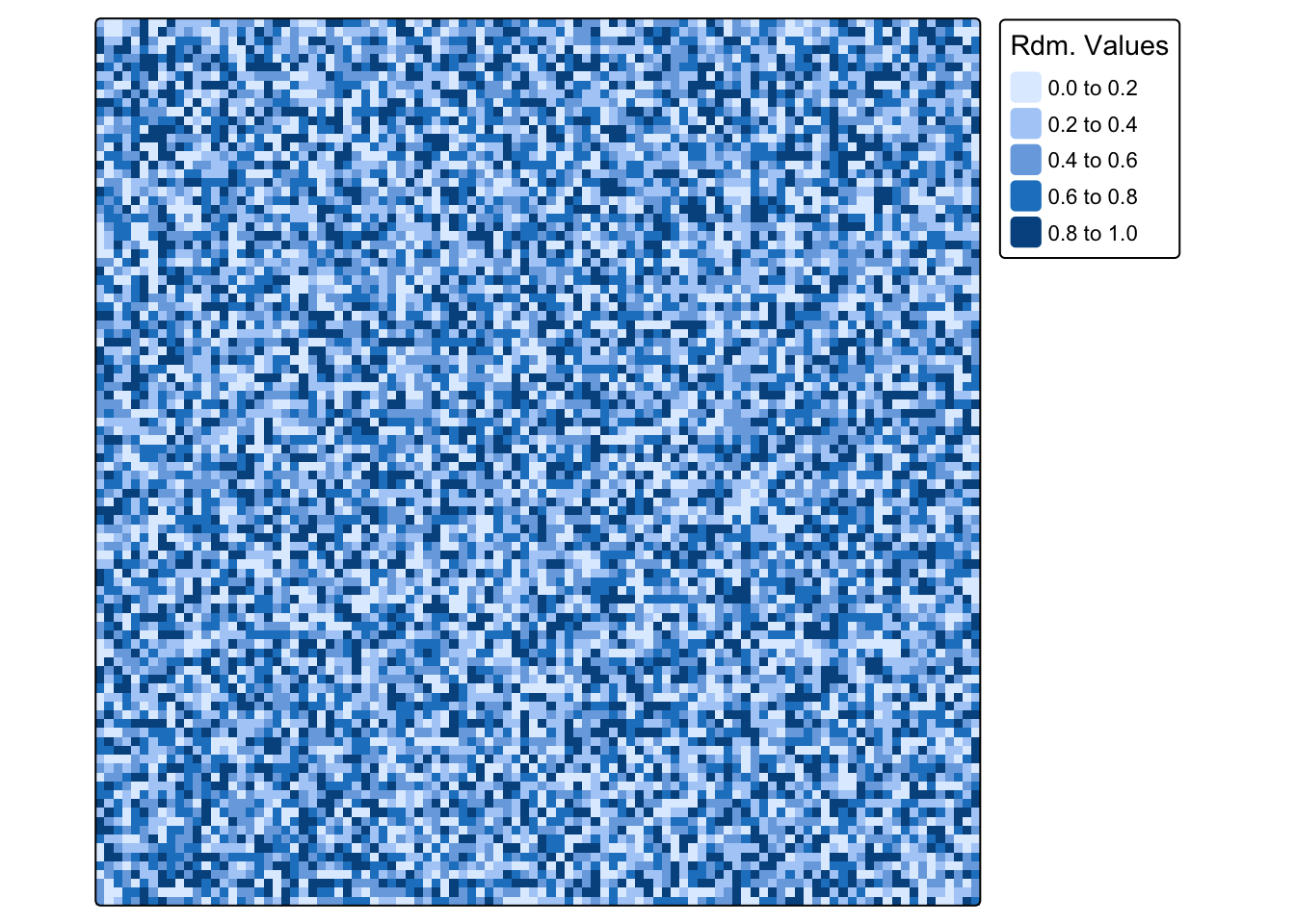
Reading spatial data from disk
The following datasets are provided as part of this practical:
Vector data
major_basins_of_the_world: POLYGON geometry ESRI Shapefile containing the major and largest drainage basins of the world. The data was obtained from the World Bank.ne_10m_populated_places: POINT geometry ESRI Shapefile containing all admin-0 and many admin-1 capitals, major cities and towns, plus a sampling of smaller towns in sparsely inhabited regions. The data is part of the Natural Earth public dataset available at 1:10 million scale.ne_110m_admin_0_countries: POLYGON geometry ESRI Shapefile containing boundaries of the countries of the world. The data is part of the Natural Earth public dataset available at 1:110 million scale.ne_110m_graticules_30: LINE geometry ESRI Shapefile containing a grid of latitude and longitude at 30 degree interval. The data is useful in illustrating map projections and is part of the Natural Earth public dataset available at 1:110 million scale.ne_110m_wgs84_bounding_box: POLYGON geometry ESRI Shapefile containing the bounding box of thene_110layers. The data is useful in illustrating map projections and is part of the Natural Earth public dataset available at 1:110 million scale.pb2002_plates: POLYGON geomtry ESRI Shapefile containing the world’s tectonic plates. The data is based on a publication in the journal G-Cubed and was downloaded from here.
Raster data
chelsa_bio12_1981-2010_V.2.1_50km: GeoTIFF raster representing mean annual precipitation for the period 1981 to 2010 derived by the CHELSA (Climatologies at high resolution for the earth’s land surface areas) project. The original raster was down-sampled to a resolution of 0.5 arc degrees (approx. 50 km at the equator) for ease of handling.
Loading data into R
Load provided data layers:
# Specify the path to your data
# Vector data
riv <- "./data/data_spat2/vector/major_basins_of_the_world.shp"
pop <- "./data/data_spat2/vector/ne_10m_populated_places.shp"
bnd <- "./data/data_spat2/vector/ne_110m_admin_0_countries.shp"
grd <- "./data/data_spat2/vector/ne_110m_graticules_30.shp"
box <- "./data/data_spat2/vector/ne_110m_wgs84_bounding_box.shp"
plt <- "./data/data_spat2/vector/pb2002_plates.shp"
# Raster data
mp <- "./data/data_spat2/raster/chelsa_bio12_1981-2010_V.2.1_50km.tif"
# Read in vectors
river_basins <- read_sf(riv)
ne_pop <- read_sf(pop)
ne_cntry <- read_sf(bnd)
ne_grid <- read_sf(grd)
ne_box <- read_sf(box)
tect_plates <- read_sf(plt)
#Read in rasters
precip <- rast(mp)
names(precip) <- "precip"Manipulating attribute data
Print the first few rows for river_basins,
ne_pop, ne_cntry, and
tect_plates:
As seen above, the ne_pop and ne_cntry
layers contain a large number of attribute columns (138 and 169,
respectively). Since we do not need all this information, we use the
following code to drop the unwanted columns and retain only the relevant
attributes:
# Keep only the columns named + the geometry column
river_basins_keep <- c("NAME", attr(river_basins, "sf_column"))
ne_pop_keep <- c("NAME", "ADM0NAME", "POP_MAX", "RANK_MAX",
attr(ne_pop, "sf_column"))
ne_cntry_keep <- c("NAME", "POP_EST", "POP_RANK", "CONTINENT",
"REGION_UN", "SUBREGION", attr(ne_cntry, "sf_column"))
tect_plates_keep <- c("PlateName", attr(tect_plates, "sf_column"))
# Use dplyr's select to keep only the desired columns
river_basins <- river_basins %>% select(all_of(river_basins_keep))
ne_pop <- ne_pop %>% select(all_of(ne_pop_keep))
ne_cntry <- ne_cntry %>% select(all_of(ne_cntry_keep))
tect_plates <- tect_plates %>% select(all_of(tect_plates_keep))
# Print rows of cleaned objects
head(river_basins)The above confirms that the unwanted attribute columns have been successfully removed.
To gain an overview of the available data, we now generate static maps to visualize the attribute columns for each vector layer.
# Identify attribute columns by excluding the geometry column
attribute_columns <- setdiff(names(ne_pop), attr(ne_pop, "sf_column"))
# Set tmap to plot mode (for static maps)
tmap_mode("plot")
# Initialize an empty list to store individual maps
map_list <- list()
# Loop over each attribute column to create maps
for (col in attribute_columns) {
# Create a map for the current attribute column
map <- tm_shape(ne_pop) +
tm_dots(size = 0.1, col) +
tm_layout(frame = FALSE) +
tm_title(paste("Map of:", col), size = 0.8) +
tm_legend(show = FALSE) +
tm_crs("+proj=mill")
# Add the map to the list (using the column name as the list element name)
map_list[[col]] <- map
}
# Arrange the individual maps into a combined layout.
# For example, here we arrange them in 2 columns.
combined_map <- do.call(tmap_arrange, c(map_list, list(ncol = 2)))
combined_map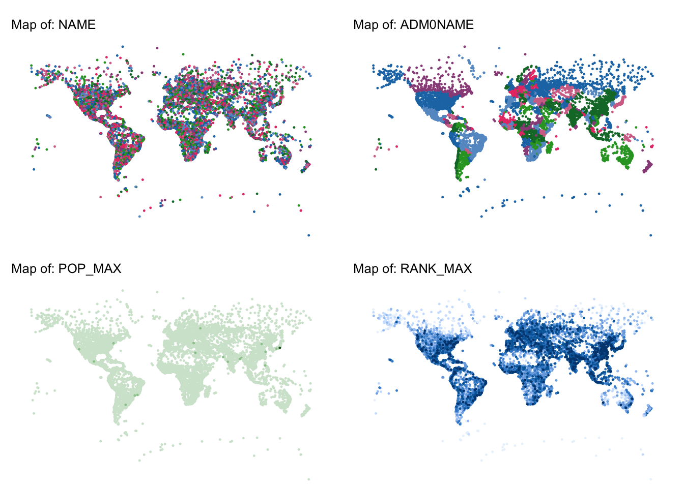
# Identify attribute columns by excluding the geometry column
attribute_columns <- setdiff(names(ne_cntry), attr(ne_cntry, "sf_column"))
# Set tmap to plot mode (for static maps)
tmap_mode("plot")
# Initialize an empty list to store individual maps
map_list <- list()
# Loop over each attribute column to create maps
for (col in attribute_columns) {
# Create a map for the current attribute column
map <- tm_shape(ne_cntry) +
tm_polygons(col) +
tm_layout(frame = FALSE) +
tm_title(paste("Map of:", col), size = 0.8) +
tm_legend(show = FALSE) +
tm_crs("+proj=mill")
# Add the map to the list (using the column name as the list element name)
map_list[[col]] <- map
}
# Arrange the individual maps into a combined layout.
# For example, here we arrange them in 3 columns.
combined_map <- do.call(tmap_arrange, c(map_list, list(ncol = 3)))
combined_map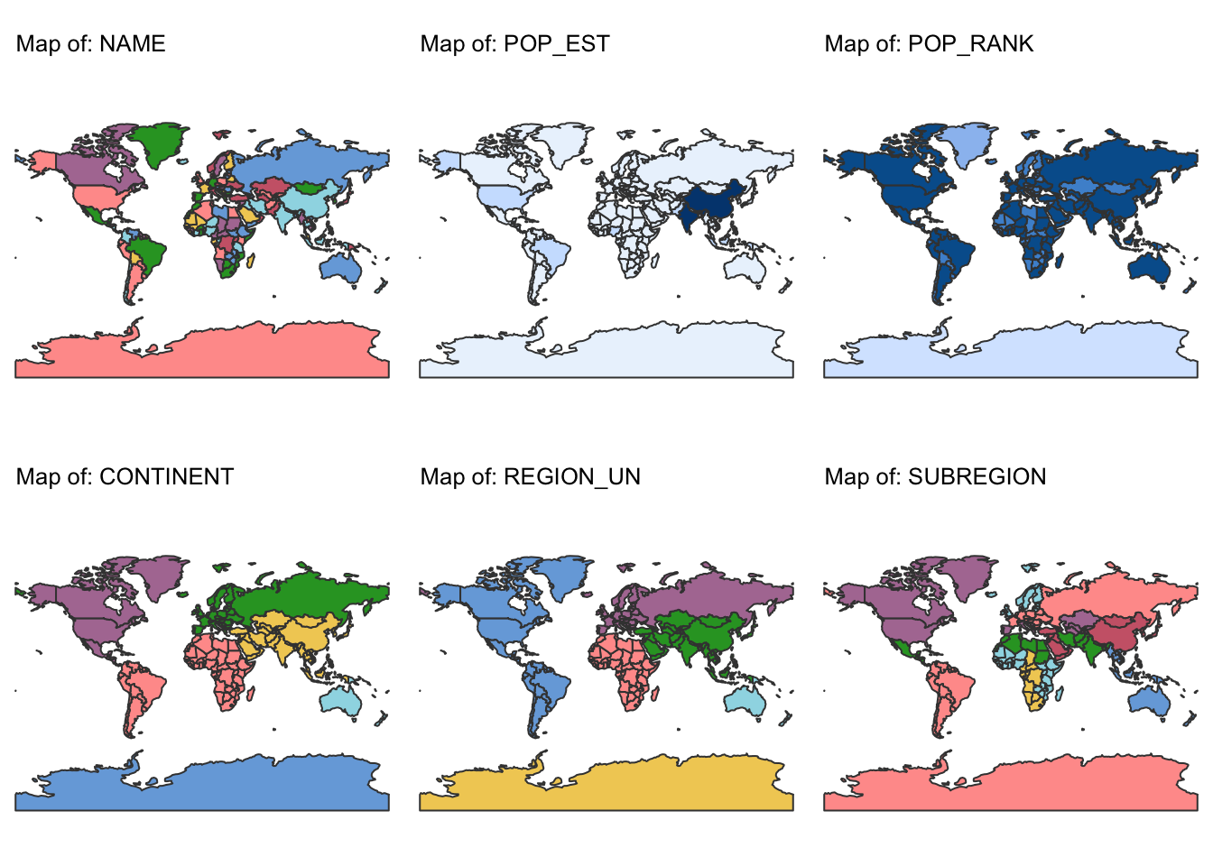
# Set tmap to plot mode (for static maps)
tmap_mode("plot")
# Plot river basins
bnd_map <- tm_shape(ne_box) + tm_borders("white")
basins_map <- bnd_map +
tm_shape(river_basins) + tm_fill("NAME") +
tm_layout(frame = FALSE) +
tm_title("Map of River Basins", size = 0.8) +
tm_legend(show = FALSE) +
tm_crs("+proj=mill")
# Plot countries on top
basins_map + tm_shape(ne_cntry) + tm_borders("gray")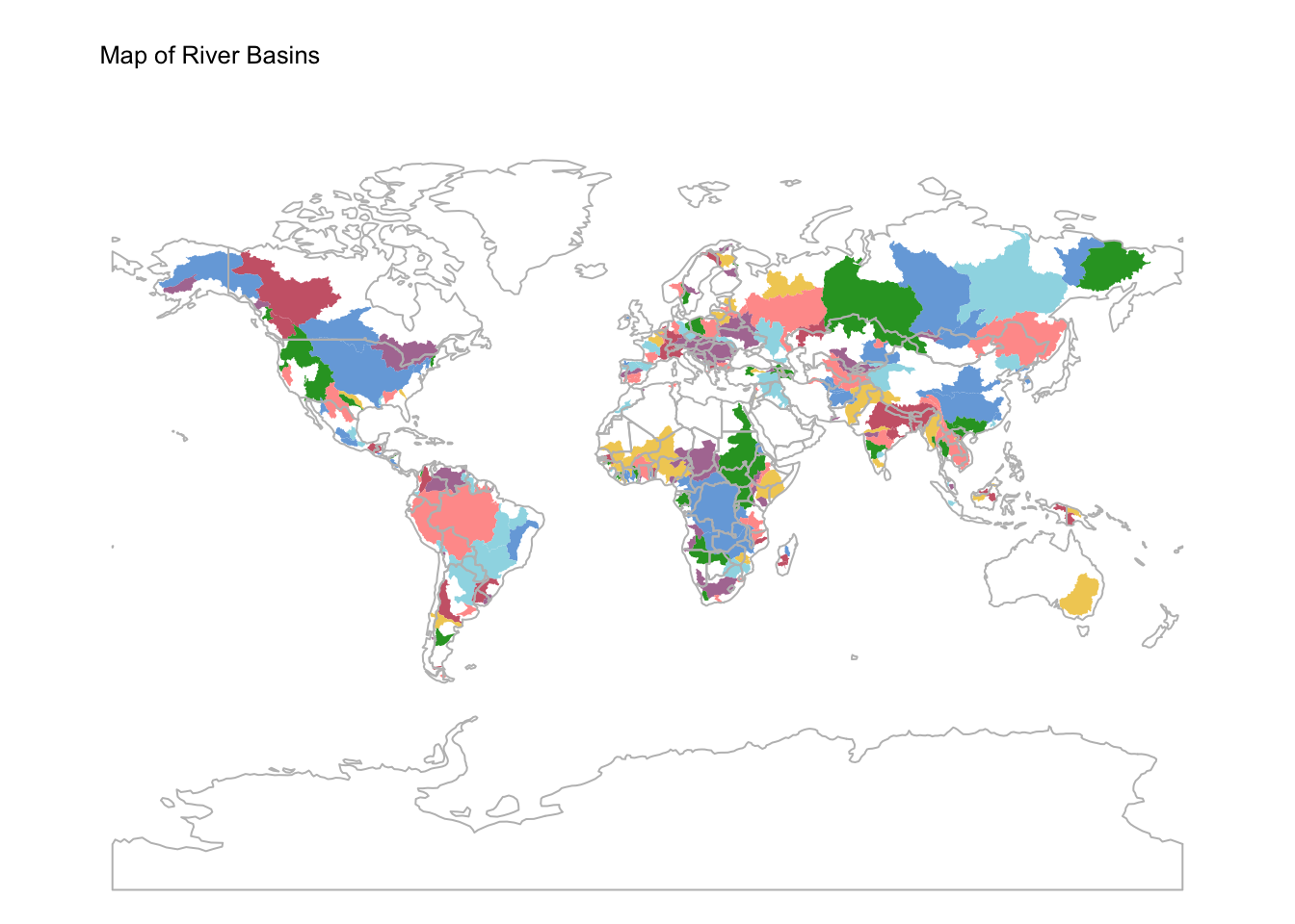
# Plot tectonic plates
plates_map <- tm_shape(tect_plates) + tm_fill("PlateName") +
tm_layout(frame = FALSE) +
tm_title("Map of Tectonic Plates", size = 0.8) +
tm_legend(show = FALSE) +
tm_crs("+proj=mill")
# Plot countries on top
plates_map + tm_shape(ne_cntry) + tm_borders("white")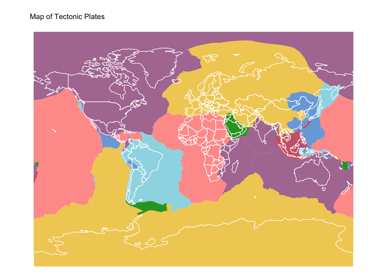
Next, plot the raster layer on a static map to inspect the extent and distribution of values, and to confirm that the data was read in correctly:
# Switch to static mode
tmap_mode("plot")
# Plot precipitation raster
rain_map <- tm_shape(precip) +
tm_raster("precip",
col.scale = tm_scale_continuous(values = "viridis"),
col.legend = tm_legend(
title = "Mean Annual \nRainfall",
position = tm_pos_out(cell.h = "right", cell.v = "center"),
orientation = "portrait"
)
) +
tm_layout(frame = FALSE) +
tm_crs("+proj=mill")
# Plot countries on top
rain_map + tm_shape(ne_cntry) + tm_borders("white")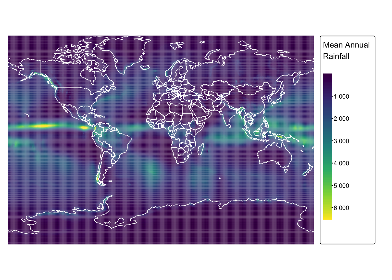
Reading data from a web service
The WFS standard
The Open Geospatial Consortium (OGC) is responsible for the global development and standardization of geospatial and location-based information. One of its key interface standards is the Web Feature Service (WFS), which enables platform-independent requests for spatial features over the internet. Unlike the Web Map Service (WMS), which delivers static map tiles, WFS provides access to vector-based spatial entities that can be queried, modified, and analysed in real-time.
This functionality is powered by Geography Markup Language (GML), an XML-based encoding standard designed to represent geographical features and their attributes. By leveraging GML, WFS allows users to interact with spatial datasets dynamically, making it an essential tool for GIS applications, spatial data sharing, and interoperability between different platforms and systems.
WFS functionality is built around three core operations:
GetCapabilities: returns a standardised, human-readable metadata document that describes the WFS service, including its available features and functionalities.DescribeFeatureType: provides a structured overview of the supported feature types, defining the schema and attributes of the available spatial data.GetFeature: enables users to retrieve specific spatial features, including their geometric representations and associated attribute values.
Accessing data via WFS in R
To access spatial data via WFS, we need to install and load two additional packages:
install.packages("httr") # Generic web-service package for working with HTTP
install.packages("ows4R") # Interface for OGC web-services incl. WFSWe will connect to the OCTOPUS database — a web-enabled database for visualizing, querying, and downloading age data and denudation rates related to erosional landscapes, Quaternary depositional landforms, and paleoecological, paleoenvironmental, and archaeological records. The OCTOPUS database stores data in a PostgreSQL/PostGIS relational database and provides access to the data via WFS.
In the next chunk of code we store the OCTOPUS WFS URL in an object, and then, using the latter, we establish a connection to the OCTOPUS database:
octopus_data <- "http://geoserver.octopusdata.org/geoserver/wfs" # Store url in object
octopus_data_client <- WFSClient$new(octopus_data, serviceVersion = "2.0.0") # Connection to dbUse getFeatureTypes() to request a list of the data
available for access from the OCTOPUS server:
The following chunk of code retrieves the data layer
be10-denude:crn_aus_basins, which contains cosmogenic
beryllium-10 denudation rates analyzed in sediment from Australian river
basins.
url <- parse_url(octopus_data) # Parse URL into list
# Set parameters for url$query
url$query <- list(service = "wfs",
version = "2.0.0",
request = "GetFeature",
typename = "be10-denude:crn_aus_basins",
srsName = "EPSG:900913")
request <- build_url(url) # Build a request URL from 'url' list
crn_aus_basins <- read_sf(request) # Read data as sf object using 'request' URL
# Print first rows of data layer
head(crn_aus_basins)The data layer is now available in R as the sf
spatial object crn_aus_basins. The table above indicates
that crn_aus_basins contains 96 attribute columns.
For the next example, we focus on two key attributes:
EBE_MMKYR– the measured denudation rate in \(mm.kyr^{-1}\)SLP_AVE– the average slope of the sampled river basins in \(m.km^{-1}\)
We use ggplot to create a scatter plot of
EBE_MMKYR versus SLP_AVE. The points are
color-coded based on elevation (ELEV_AVE) and scaled
according to basin area (AREA).
# Plot denudation rate over average slope
my_plot <-
ggplot(crn_aus_basins, aes(x=SLP_AVE, y=EBE_MMKYR)) +
# Show error bars
geom_errorbar(aes(ymin=(EBE_MMKYR-EBE_ERR), ymax=(EBE_MMKYR+EBE_ERR)),
linewidth=0.3, colour="gray80") +
# Scale pts. to "AREA", colour pts. to "ELEV_AVE"
# Define point size range for better visibility
geom_point(aes(size=AREA, color=ELEV_AVE), alpha=.4) +
scale_size_continuous(range = c(1, 12)) +
# Set labels for x and y axes
xlab("Slope gradient [m/km]") +
ylab("Denudation rate [mm/kyr]") +
# Add title
ggtitle("Denudation rates [mm/kyr]") +
# Legend
labs(size = "Basin \narea [km^2]",
colour = "Average \nbasin \nelevation [m]")
my_plot # Make plot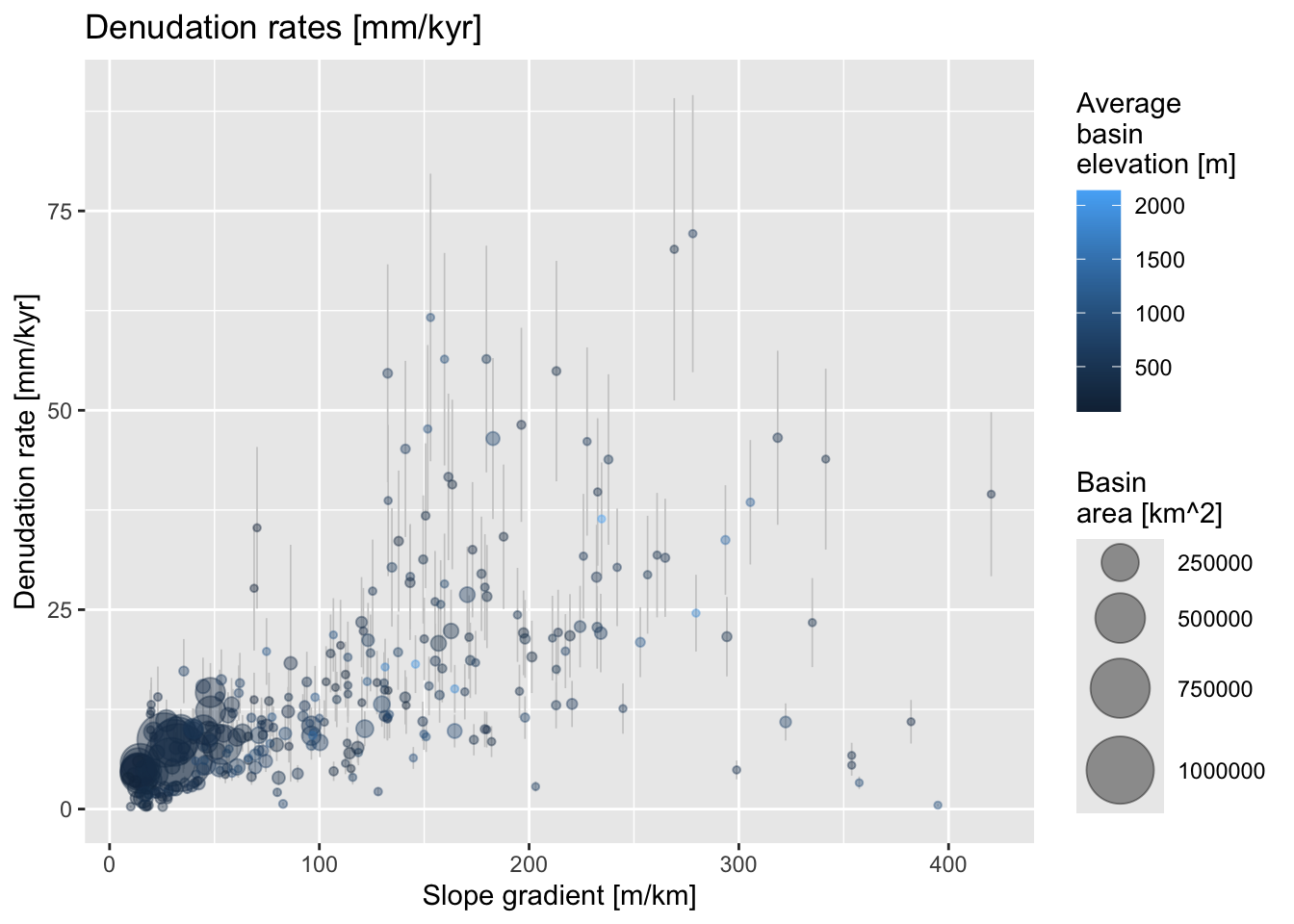
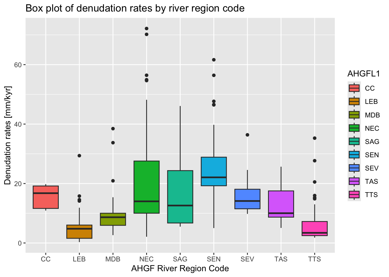
We can also produce a box plot showing denudation rates grouped by
the AHGF
river region code (column AHGFL1):
ggplot(crn_aus_basins,
aes(x = AHGFL1,
y = EBE_MMKYR,
fill = AHGFL1)
) +
geom_boxplot() +
labs(
title = "Box plot of denudation rates by river region code",
x = "AHGF River Region Code",
y = "Denudation rates [mm/kyr]"
)
In the following example, we plot a subset of the
crn_aus_basins data on an interactive map. The dataset is
grouped by individual studies, identified using the STUDYID
column. We extract one of these studies (STUDYID = “S252”)
and color the resulting basins based on denudation rates
(EBE_MMKYR) to visualize their distribution.
Before mapping, we need to convert the crn_aus_basins
spatial object to POLYGON geometry. Although the river basins are
inherently polygons, the dataset is downloaded from the OCTOPUS server
with its geometry defined as MULTISURFACE, which is incompatible with
tmap. We resolve this issue using the
st_cast() function.
Next, we re-project the data to WGS 84 coordinates to avoid
plotting issues. Finally, we filter the dataset to retain only records
where STUDYID equals “S252”, removing all other
entries.
# Loaded polygon object in as MULTISURFACE and needs converting
# to POLYGON before plotting
crn_aus_basins <-st_cast(crn_aus_basins, "GEOMETRYCOLLECTION") %>%
st_collection_extract("POLYGON")
# If the above fails, save as ESRI shapefile
# This will force geometry to be POLYGON:
# st_write(crn_aus_proj, "./data/crn_aus.shp", delete_dsn = TRUE)
# crn_aus_poly <- read_sf("./data/crn_aus.shp")
crn_aus_basins <- st_set_crs(crn_aus_basins, 900913)
crn_aus_proj = st_transform(crn_aus_basins, crs = "EPSG:4326")
# Drop all basins with the exception of those with STUDYID = S252
crn_aus_s252 = crn_aus_proj |>
filter(STUDYID %in% "S252")
# Drop columns and only keep OBSID2 and EBE_MMKYR
crn_aus_s252_keep <- c("OBSID2", "EBE_MMKYR", attr(crn_aus_s252, "sf_column"))
crn_aus_s252 <- crn_aus_s252 %>% select(all_of(crn_aus_s252_keep))
#Switch to interactive mode
tmap_mode("view")
#Plot basins
tm_shape(crn_aus_s252) +
tm_polygons(fill = "EBE_MMKYR",
fill.scale = tm_scale_continuous(values = "-scico.roma"),
fill_alpha = 0.4)In summary, spatial data loaded into R via WFS behaves in the same way as spatial data loaded from disk. Once imported, it can be manipulated using the same sf and terra functions as locally stored spatial datasets. This includes performing spatial joins, transformations, filtering, aggregations, and visualizations. WFS-loaded data can also be saved to disk. Another advantage of working with WFS is that it enables access to live, updated spatial datasets hosted by different organizations, reducing the need for manual downloads. However, since WFS data is fetched remotely, users should be mindful of network latency and potential server limitations when working with large datasets.
Coordinate systems
This section provides an introduction to coordinate reference systems (CRS) and explores the fundamental concepts of CRS transformations in R.
A CRS is a framework used to define locations on the Earth’s surface by providing a standardised method for mapping geographic coordinates (latitude and longitude) onto a two-dimensional plane. A CRS consists of a datum, which establishes a reference model of the Earth’s shape, an ellipsoid, which approximates the Earth’s surface, and a projection, which translates the three-dimensional Earth onto a flat surface.
There are two primary types of coordinate reference systems:
geographic coordinate systems (GCS), which use a spherical coordinate system based on latitude and longitude, and
projected coordinate systems (PCS), which apply mathematical transformations to represent the curved surface on a flat plane, enabling easier distance and area calculations.
The main types of map projections are classified based on the properties they preserve:
conformal projections, such as the Mercator projection, preserve local angles and shapes but distort size, making them useful for navigation.
equal-area projections, like the Albers or Mollweide projections, maintain area proportions while distorting shapes, making them ideal for statistical and thematic maps.
equidistant projections, such as the Azimuthal Equidistant projection, preserve distances from a central point, benefiting applications like radio transmission mapping.
compromise projections, such as the Robinson or Winkel Tripel projections, balance shape and area distortions to create visually appealing world maps.
The choice of projection depends on the intended use and geographic region of interest, as every projection introduces some form of distortion due to the challenge of flattening a curved surface.
Handling CRS information in R
In R, projections are managed using a suite of geospatial packages — including but not limited to sf and terra — that leverage external libraries like PROJ and GDAL for handling coordinate systems and CRS transformations.
Defining or identifying a CRS in R can be done using three main approaches:
Using a PROJ string
A PROJ string is a textual representation that
explicitly defines the parameters of a coordinate reference system. This
string consists of a series of key-value pairs prefixed with the
+ character, that describe various aspects of the CRS,
including the projection type, datum, central meridian, standard
parallels, and other essential transformation parameters. For
example:
+proj=aea +lat_1=0 +lat_2=-30 +lon_0=130defines an Albers Equal Area (AEA) projection, specifying two standard parallels at 0 and -30 degrees latitude and a central meridian at 130 degrees longitude.+proj=robindefines a Robinson projection, commonly used for world maps. When no other parameters are provided, the CRS transformation will use the default values of all missing parameters. A more complete PROJ string syntax for identifying the Robinson projection would be:+proj=robin +lon_0=0 +x_0=0 +y_0=0 +ellps=WGS84 +datum=WGS84 +units=m +no_defs.
The PROJ string method is becoming deprecated and using ‘authority:code’ strings or Well-Known Text (WKT) formats (see below) is recommended.
Using a WKT-CRS string
Well-Known Text (WKT) is a standardised text format for representing
CRS information, providing a structured and comprehensive way to define
projection parameters, datums, and coordinate systems. Unlike the older
PROJ strings, which use a simplified notation with
+proj= parameters, WKT offers a more
descriptive, human-readable, and machine-interpretable format.
WKT structured CRS information may be embedded in a metadata file.
Below is and example of a WKT-CRS representation of the WGS 84
geographic coordinate system embeded in the river_basins sf
object:
GEOGCRS["WGS 84",
DATUM["World Geodetic System 1984",
ELLIPSOID["WGS 84", 6378137, 298.257223563,
LENGTHUNIT["metre", 1]]
],
PRIMEM["Greenwich", 0,
ANGLEUNIT["degree", 0.0174532925199433]
],
CS[ellipsoidal, 2],
AXIS["latitude", north,
ORDER[1],
ANGLEUNIT["degree", 0.0174532925199433]
],
AXIS["longitude", east,
ORDER[2],
ANGLEUNIT["degree", 0.0174532925199433]
],
ID["EPSG", 4326]
]The above WKT representation clearly defines the datum (WGS 84), ellipsoid parameters, prime meridian, coordinate axes, and the EPSG authority code (EPSG:4326).
In sf the function st_crs() retrieves
or assigns a CRS to a spatial object, while st_transform()
converts it to a different projection. Similarly, in the
terra package, the crs() function is used
to check or assign projections, and project() re-projects
raster data to a new CRS.
Both sf and terra accept both PROJ strings and EPSG codes. Further, both sf and terra handle WKT natively:
# sf package
# Retrieve the CRS in WKT format for an sf object
crs_wkt <- st_crs(river_basins)$wkt
# Print WKT representation
print(crs_wkt)## [1] "GEOGCRS[\"WGS 84\",\n DATUM[\"World Geodetic System 1984\",\n ELLIPSOID[\"WGS 84\",6378137,298.257223563,\n LENGTHUNIT[\"metre\",1]]],\n PRIMEM[\"Greenwich\",0,\n ANGLEUNIT[\"degree\",0.0174532925199433]],\n CS[ellipsoidal,2],\n AXIS[\"latitude\",north,\n ORDER[1],\n ANGLEUNIT[\"degree\",0.0174532925199433]],\n AXIS[\"longitude\",east,\n ORDER[2],\n ANGLEUNIT[\"degree\",0.0174532925199433]],\n ID[\"EPSG\",4326]]"# terra package
# Retrieve the CRS in WKT format for an SpatRaster object
crs_wkt <- crs(precip)
# Print WKT representation
print(crs_wkt)## [1] "GEOGCRS[\"WGS 84\",\n ENSEMBLE[\"World Geodetic System 1984 ensemble\",\n MEMBER[\"World Geodetic System 1984 (Transit)\"],\n MEMBER[\"World Geodetic System 1984 (G730)\"],\n MEMBER[\"World Geodetic System 1984 (G873)\"],\n MEMBER[\"World Geodetic System 1984 (G1150)\"],\n MEMBER[\"World Geodetic System 1984 (G1674)\"],\n MEMBER[\"World Geodetic System 1984 (G1762)\"],\n MEMBER[\"World Geodetic System 1984 (G2139)\"],\n MEMBER[\"World Geodetic System 1984 (G2296)\"],\n ELLIPSOID[\"WGS 84\",6378137,298.257223563,\n LENGTHUNIT[\"metre\",1]],\n ENSEMBLEACCURACY[2.0]],\n PRIMEM[\"Greenwich\",0,\n ANGLEUNIT[\"degree\",0.0174532925199433]],\n CS[ellipsoidal,2],\n AXIS[\"geodetic latitude (Lat)\",north,\n ORDER[1],\n ANGLEUNIT[\"degree\",0.0174532925199433]],\n AXIS[\"geodetic longitude (Lon)\",east,\n ORDER[2],\n ANGLEUNIT[\"degree\",0.0174532925199433]],\n USAGE[\n SCOPE[\"Horizontal component of 3D system.\"],\n AREA[\"World.\"],\n BBOX[-90,-180,90,180]],\n ID[\"EPSG\",4326]]"You can also define a new CRS using a WKT string and then assign to a spatial object:
# Define WKT
wkt_string <- 'GEOGCRS["WGS 84",
ENSEMBLE["World Geodetic System 1984 ensemble",
MEMBER["World Geodetic System 1984 (Transit)"],
MEMBER["World Geodetic System 1984 (G730)"],
MEMBER["World Geodetic System 1984 (G873)"],
MEMBER["World Geodetic System 1984 (G1150)"],
MEMBER["World Geodetic System 1984 (G1674)"],
MEMBER["World Geodetic System 1984 (G1762)"],
MEMBER["World Geodetic System 1984 (G2139)"],
ELLIPSOID["WGS 84", 6378137, 298.257223563,
LENGTHUNIT["metre", 1]],
ENSEMBLEACCURACY[2.0]
],
PRIMEM["Greenwich", 0,
ANGLEUNIT["degree", 0.0174532925199433]
],
CS[ellipsoidal, 2],
AXIS["geodetic latitude (Lat)", north,
ORDER[1],
ANGLEUNIT["degree", 0.0174532925199433]
],
AXIS["geodetic longitude (Lon)", east,
ORDER[2],
ANGLEUNIT["degree", 0.0174532925199433]
],
USAGE[
SCOPE["Horizontal component of 3D system."],
AREA["World."],
BBOX[-90, -180, 90, 180]
],
ID["EPSG", 4326]
]'
# Assign WKT to raster
crs(precip) <- wkt_stringUsing WKT-CRS representations provides significant flexibility. However, in practice, using EPSG/ESRI codes (or even PROJ strings) is often more straightforward and produces the desired results.
CRS transformations in R
Projecting vector data
Below, we re-project the ne_cntry sf
object to the Eckert IV coordinate reference system (CRS) using
the three approaches discussed earlier for defining a CRS: PROJ
strings, EPSG/ESRI codes, and WKT-CRS
strings.
cntry_eck4_1 = st_transform(ne_cntry, crs = "+proj=eck4") # PROJ string
cntry_eck4_2 = st_transform(ne_cntry, crs = "ESRI:54012") # ESRI authority code
# Define WKT
wkt_string_eck4 <- 'PROJCS["World_Eckert_IV",
GEOGCS["WGS 84",
DATUM["WGS_1984",
SPHEROID["WGS 84",6378137,298.257223563,
AUTHORITY["EPSG","7030"]],
AUTHORITY["EPSG","6326"]],
PRIMEM["Greenwich",0],
UNIT["Degree",0.0174532925199433]],
PROJECTION["Eckert_IV"],
PARAMETER["central_meridian",0],
PARAMETER["false_easting",0],
PARAMETER["false_northing",0],
UNIT["metre",1,
AUTHORITY["EPSG","9001"]],
AXIS["Easting",EAST],
AXIS["Northing",NORTH],
AUTHORITY["ESRI","54012"]]'
cntry_eck4_3 = st_transform(ne_cntry, crs = wkt_string_eck4) # WKT string
#Switch to static mode
tmap_mode("plot")
# Plot re-projected layers + grid and bounding box
map1 <- tm_shape(cntry_eck4_1) +
tm_borders(col = "black") +
tm_layout(frame = FALSE) +
tm_title("PROJ string", size = 1)
map1b <- map1 +
tm_shape(ne_grid) + tm_lines(col = "darkred", lwd = 0.4)
map1c <- map1b + tm_shape(ne_box) + tm_borders(col = "darkred", lwd = 0.4)
map2 <- tm_shape(cntry_eck4_2) +
tm_borders(col = "black") +
tm_layout(frame = FALSE) +
tm_title("EPSG/ESRI code", size = 1)
map2b <- map2 +
tm_shape(ne_grid) + tm_lines(col = "darkred", lwd = 0.4)
map2c <- map2b + tm_shape(ne_box) + tm_borders(col = "darkred", lwd = 0.4)
map3 <- tm_shape(cntry_eck4_3) +
tm_borders(col = "black") +
tm_layout(frame = FALSE) +
tm_title("WKT string", size = 1)
map3b <- map3 +
tm_shape(ne_grid) + tm_lines(col = "darkred", lwd = 0.4)
map3c <- map3b + tm_shape(ne_box) + tm_borders(col = "darkred", lwd = 0.4)
tmap_arrange(map1c, map2c, map3c)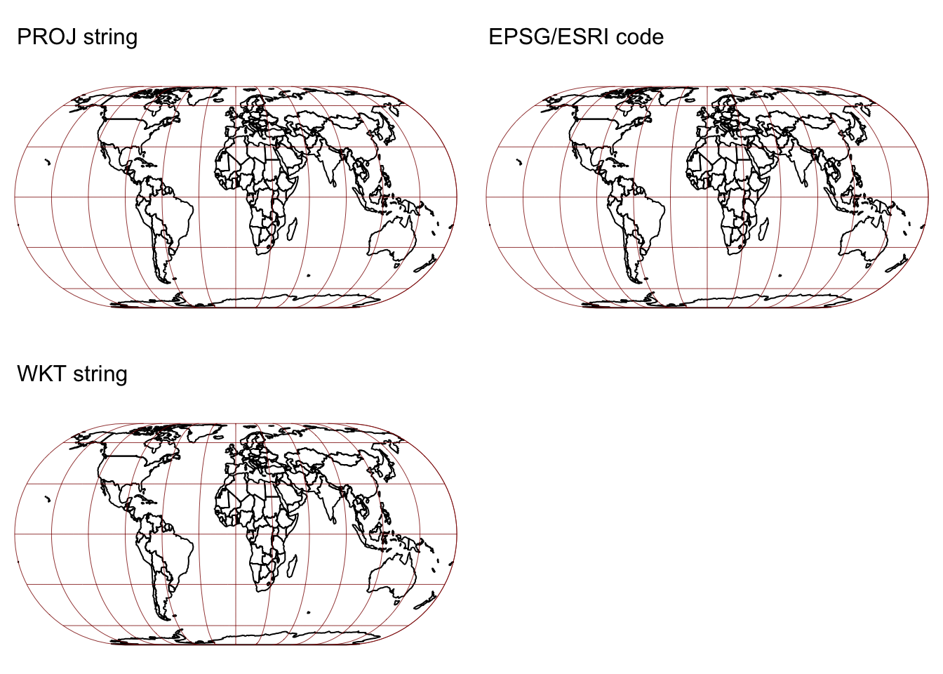
As expected all three approaches work and produce the same result.
Next, we use PROJ strings to modify the projection parameters, specifically by changing the central meridian’s value from 0 to a different longitude. This effectively “rotates” the map, centering it on the newly defined central meridian. The same “customisation” is achievable using a modified WTK-CRS string, however, it is not possible when using EPSG/ESRI codes!
To ensure the spatial object is correctly re-projected in R, any
features that intersect the antimeridian (i.e., the +/-180 degree
longitude line, directly opposite the central meridian) must be split at
that boundary. This is accomplished using the
st_break_antimeridian() function. If these intersecting
features are not split, R will be unable to correctly position them,
causing them to appear as stripes on the map.
# Define new meridian
meridian1 <- -69
meridian2 <- 150
# Split world at new meridian
ne_cntry_split1 <- st_break_antimeridian(ne_cntry, lon_0 = meridian1)
ne_cntry_split2 <- st_break_antimeridian(ne_cntry, lon_0 = meridian2)
# Re-project without breaking features at antimeridian to show problem
cntry_eck4_0 <- st_transform(ne_cntry,
paste("+proj=eck4 +lon_0=", meridian1 ,
"+k=1 +x_0=0 +y_0=0 +ellps=WGS84 +datum=WGS84 +units=m +no_defs"))
# Now re-project using new meridian center
cntry_eck4_1 <- st_transform(ne_cntry_split1,
paste("+proj=eck4 +lon_0=", meridian1 ,
"+k=1 +x_0=0 +y_0=0 +ellps=WGS84 +datum=WGS84 +units=m +no_defs"))
cntry_eck4_2 <- st_transform(ne_cntry_split2,
paste("+proj=eck4 +lon_0=", meridian2 ,
"+k=1 +x_0=0 +y_0=0 +ellps=WGS84 +datum=WGS84 +units=m +no_defs"))
#Switch to static mode
tmap_mode("plot")
# Plot re-projected layers + grid and bounding box
map0 <- tm_shape(cntry_eck4_0) +
tm_borders(col = "black") +
tm_layout(frame = FALSE) +
tm_title("Central meridian = -69 \nFeatures not broken at antimeridian", size = 1)
map1 <- tm_shape(cntry_eck4_1) +
tm_borders(col = "black") +
tm_layout(frame = FALSE) +
tm_title("Central meridian = -69 \nFeatures broken and plotting correctly", size = 1)
map2 <- tm_shape(cntry_eck4_2) +
tm_borders(col = "black") +
tm_layout(frame = FALSE) +
tm_title("Central meridian = 150", size = 1)
tmap_arrange(map0, map1, map2)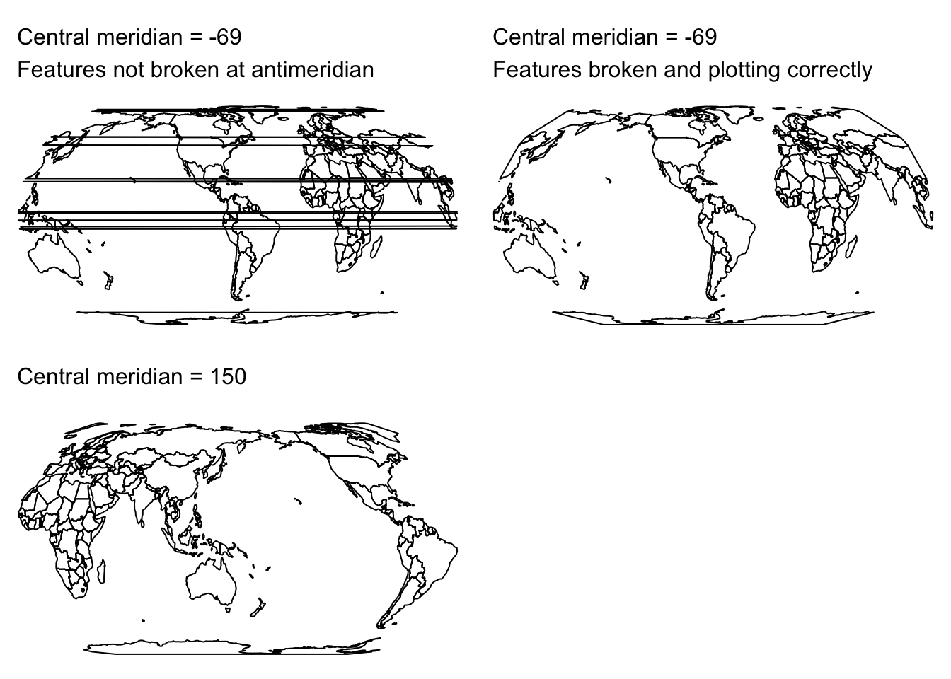
Projecting raster data
When projecting a vector layer, each geometric coordinate (points, lines, polygons) is mathematically transformed from one coordinate system to another. This process preserves the exact geometry without introducing sampling errors. In contrast, when projecting a raster layer, the entire grid of pixels must be re-sampled to align with the new coordinate system. This re-sampling can lead to slight distortions or a loss of resolution. It is therefore important that the right re-sampling (interpolation) method is used:
The three main available re-sampling methods are:
Nearest neighbor: This method selects the closest pixel value from the original grid. It’s computationally fast and preserves the original data values, making it ideal for categorical data (like land cover classifications). However, it can produce a “blocky” appearance in continuous data.
Bilinear interpolation: This method calculates the new pixel value by averaging the values of the four nearest cells, weighted by distance. It smooths out the transitions between pixels and is generally preferred for continuous data (such as temperature or elevation), though it may slightly alter the original values.
Cubic convolution: This more advanced technique considers 16 neighboring pixels, resulting in even smoother transitions. While it provides visually appealing results, it may blur the data slightly, which could be a drawback depending on your application.
Other factors to consider when projecting raster data, include:
Resolution and extent: The output raster may have a different cell size and overall extent compared to the original. Careful selection of these parameters is essential to balance detail preservation and computational efficiency. As a rule, the resolution of the re-projected raster should not be higher (i.e., smaller pixel size) than that of the inpur raster.
Data integrity: Each interpolation method introduces its own form of approximation. For continuous data, this means a potential loss of detail or slight distortions, while for categorical data, choosing the wrong method can lead to misclassification.
Processing time and resources: More complex interpolation methods like cubic convolution require additional computation, which may impact processing time, especially with large datasets.
The above means that when projecting raster data, the
project() function in terra requires
additional parameters that include the resolution of the output raster
and the re-sampling method. When these additional parameters are not
given, project() will try to guess the most appropriate
values based on the properties of the input raster.
Below, we re-project the precip raster, which was
previously loaded into R, from the WGS 84 geographic CRS to the
Goode Homolosine (ESRI:54052) CRS.
precip_goode <- project(precip, # Raster to be projected
"ESRI:54052", # Output CRS
method = "bilinear", # Re-sampling method
res = 50000) # Resolution
# Switch to static mode
tmap_mode("plot")
# Plot precipitation raster
rain_map <- tm_shape(precip_goode) +
tm_raster("precip",
col.scale = tm_scale_continuous(values = "viridis"),
col.legend = tm_legend(
title = "Mean Annual \nRainfall",
position = tm_pos_out(cell.h = "right", cell.v = "center"),
orientation = "portrait"
)
) +
tm_layout(frame = FALSE) + tm_title("Goode Homolosine (ESRI:54052)", size = 1)
# Plot countries on top
rain_map + tm_shape(ne_cntry) + tm_borders("white")
Next, we re-project again, changing the re-sampling method to
near (nearest neighbor) and output resolution to 500
km:
precip_goode <- project(precip, # Raster to be projected
"ESRI:54052", # Output CRS
method = "near", # Re-sampling method
res = 500000) # Resolution
# Switch to static mode
tmap_mode("plot")
# Plot precipitation raster
rain_map <- tm_shape(precip_goode) +
tm_raster("precip",
col.scale = tm_scale_continuous(values = "viridis"),
col.legend = tm_legend(
title = "Mean Annual \nRainfall",
position = tm_pos_out(cell.h = "right", cell.v = "center"),
orientation = "portrait"
)
) +
tm_layout(frame = FALSE) + tm_title("Goode Homolosine (ESRI:54052)", size = 1)
# Plot countries on top
rain_map + tm_shape(ne_cntry) + tm_borders("white")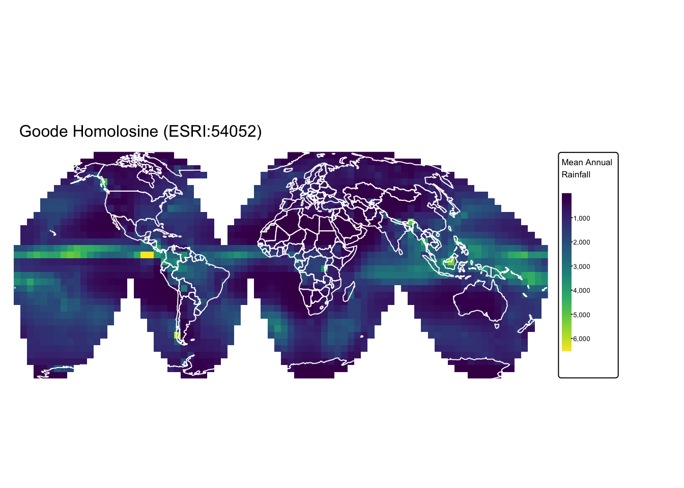
Geoprocessing operations
Basic geospatial operations involve handling vector and raster data to analyze and manipulate spatial features. Vector data, which represent discrete entities as points, lines, and polygons, support operations that include:
Spatial queries retrieve geographic features based on specific location criteria, such as proximity, containment, or intersection. They enable users to filter and analyze spatial data by formulating queries that consider the relationships between different features.
Buffering generates zones around spatial features at a designated distance, facilitating proximity analysis and risk assessment. This operation helps identify all features within a certain distance from points, lines, or polygons, which is useful for planning and environmental studies.
Overlay analysis combines two or more spatial layers to discover relationships between features and generate new data outputs. By performing operations like intersection, union, or difference, it integrates diverse datasets to provide insights into spatial patterns and interactions.
Topological operations enforce rules that define the spatial relationships between vector features, ensuring connectivity, adjacency, and containment are maintained. These processes preserve data integrity by preventing issues such as overlapping boundaries or gaps between adjacent features.
Key geospatial operations for raster data include map algebra, reclassification, and zonal statistics:
Map algebra applies mathematical operations to raster data by performing cell-by-cell calculations, allowing the derivation of new spatial information such as gradients or vegetation indices. This method supports complex analyses, enabling the modeling of environmental processes and the transformation of raw data into meaningful layers.
Reclassification transforms raster values into simplified, more interpretable classes by grouping or assigning new categories based on specified criteria. This process streamlines data analysis by converting continuous data into discrete segments, which facilitates pattern recognition and decision-making.
Zonal statistics compute summary metrics—such as the mean, sum, or maximum—of raster values within defined vector zones. This operation integrates raster and vector datasets, providing localized insights that are essential for applications like resource management and urban planning.
Spatial query
Selecting by location
Selecting by location involves filtering features based on their spatial relationship with a given geometry. The sf package provides a suite of spatial functions such as:
st_intersects(): This function returnsTRUEwhen two geometries share any part of space, meaning they have at least one point in common. It is essential in spatial queries to determine if features overlap or touch.st_disjoint(): This function is the opposite ofst_intersect()and returnsTRUEwhen two geometries do not share any points at all. It is used to identify features that are completely separate, ensuring there is no spatial overlap.st_within(): This function checks whether one geometry is entirely contained within another, meaning every point of the first lies inside the second. It is commonly applied in spatial analyses to determine hierarchical relationships, such as whether a smaller area is fully within a larger boundary.st_contains(): This function returnsTRUEwhen one geometry completely encloses another, serving as the complement tost_within(). When the arguments are swapped, it is equivalent tost_within()with reversed parameters, providing flexibility in spatial queries.
The following examples, illustrate how these functions work.
Example 1: Countries that are drained by the river Nile.
In this example, we use the st_intersects() function to
extract all countries from ne_cntry and all populated
places from ne_pop that intersect the Nile River basin in
river_basins. Before applying st_intersects(),
we first filter the river_basins sf object
to isolate the polygon representing the Nile basin.
It is important to note that, since ne_pop has
POINT geometry, both st_intersects() and
st_within() will yield the same result. However, this is
not the case for LINE and POLYGON
geometries, where the two functions produce different outputs (see
Example 3 below).
# Drop all basins with the exception of the Nile
nile = river_basins |>
filter(NAME %in% "Nile")
# Select countries that intersect the Nile
# st_intersects() with sparse = FALSE returns a matrix of logical values
# (rows: countries, columns: Nile parts)
# apply(..., 1, any) reduces each row to TRUE if any intersection exists,
# creating a logical vector for subsetting.
cntry_nile <- ne_cntry[apply(st_intersects(ne_cntry, nile, sparse = FALSE), 1, any), ]
# Select cities and towns that intersect the Nile
pop_nile <- ne_pop[apply(st_intersects(ne_pop, nile, sparse = FALSE), 1, any), ]
# Plot countries and cities intersecting the Nile
cntry_map <- tm_shape(cntry_nile) +
tm_polygons("NAME") +
tm_layout(frame = FALSE) +
tm_title("Countries intersecting the Nile basin", size = 1)
nile_map <- cntry_map +
tm_shape(nile) + tm_borders(col = "darkred", lwd = 2)
nile_map + tm_shape(pop_nile) + tm_dots(size = 0.25, col = "black")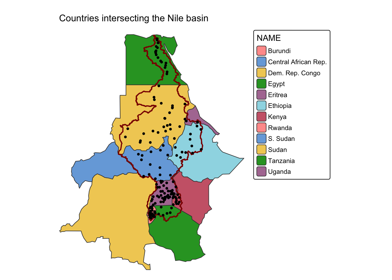
Example 2: Countries that are not drained by the river Nile.
In this example, we use st_disjoint() to select all
African countries that are not drained by the Nile River. Before
applying st_disjoint(), we first filter
ne_cntry to retain only countries located in Africa. This
ensures that the operation is performed exclusively within the relevant
geographic region.
# Drop all countries with the exception of those in Africa
africa = ne_cntry |>
filter(CONTINENT %in% "Africa")
# Select countries that do not intersect the Nile
cntry_not_nile <- africa[st_disjoint(africa, nile, sparse = FALSE), ]
# Plot countries that do not intersect the Nile
tm_shape(cntry_not_nile) +
tm_polygons("SUBREGION") +
tm_layout(frame = FALSE) +
tm_title("Countries not intersecting the Nile basin", size = 1)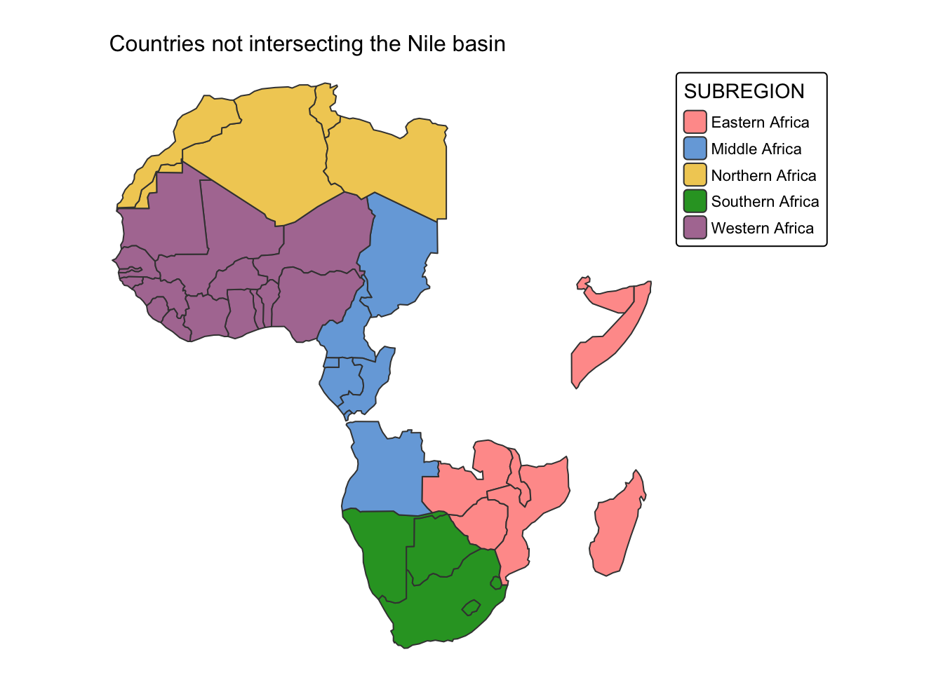
Example 3: Countries that are completely within the Danube River basin
In this example, we use st_within() to select countries
from ne_cntry that are entirely within the Danube River’s
drainage basin. Additionally, to enhance the map, we use
st_intersects() to extract countries that are partially
drained by the Danube but not fully contained within its drainage basin.
These partially drained countries are highlighted in gray.
# Drop all basins with the exception of the Danube
danube = river_basins |>
filter(NAME %in% "Danube")
# Select countries that are fully within the Danube basin
cntry_danube_within <-
ne_cntry[apply(st_within(ne_cntry, danube, sparse = FALSE), 1, any), ]
# Also select countries that intersect the Danube basin
cntry_danube_intersect <-
ne_cntry[apply(st_intersects(ne_cntry, danube, sparse = FALSE), 1, any), ]
# Plot countries that are fully within the Danube basin
cntry_map <-
tm_shape(cntry_danube_intersect) +
tm_fill("lightgray") +
tm_borders(col = "darkgray", lwd = 0.5)
danube_map <- cntry_map +
tm_shape(danube) + tm_borders(col = "darkred", lwd = 2)
danube_map +
tm_shape(cntry_danube_within) +
tm_polygons("NAME") +
tm_layout(frame = FALSE) +
tm_title("Countries completely within the Danube basin", size = 1)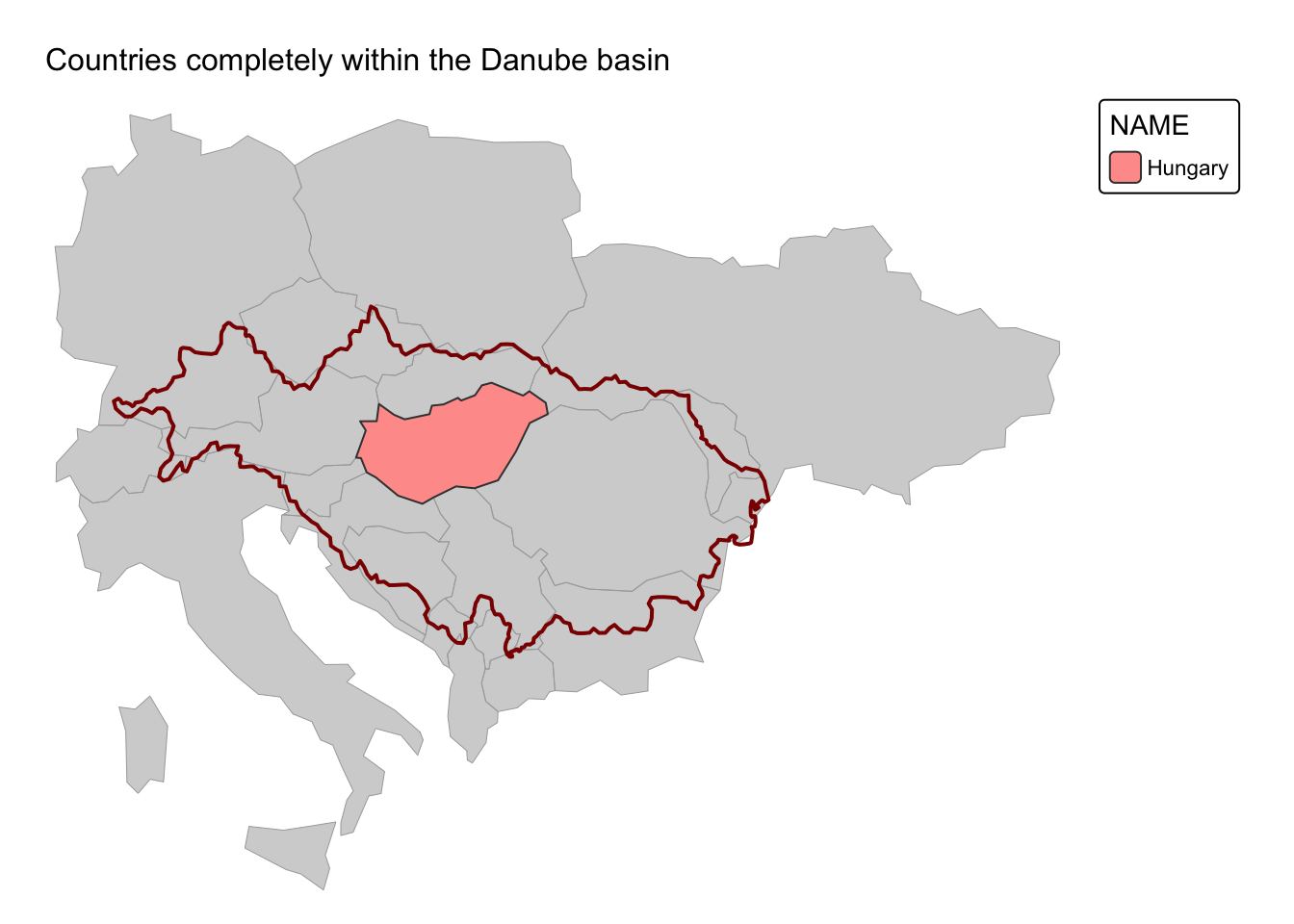
Spatial join
Spatial joins combine attributes from two sf objects
based on their spatial relationships. The st_join()
function performs a join using a specified spatial predicate. For
instance, you might join point data with polygon data to associate each
point with the attributes of the polygon it falls in.
If you need to join or select features that do not
intersect (i.e., are spatially separate), you can use
st_disjoint() as the join predicate. This effectively
provides the complement of an intersection-based join.
In the following example, we join ne_pop with
river_basins, ensuring that each populated place located
within a major river basin is assigned the name of that river basin in a
new attribute column:
# Join polygon attributes to each point that falls within a polygon
ne_pop_join <- st_join(ne_pop, river_basins, join = st_intersects)
# Print new layer's attribute table
head(ne_pop_join)As shown above, ne_pop now includes a new attribute
column, NAME.y, which stores the names of river basins for
the ne_pop points that fall within one of the polygons in
river_basins.
To rename this column to something more meaningful, you can use the following approach:
# Rename joined columns for clarity
colnames(ne_pop_join)[which(colnames(ne_pop_join) %in% c("NAME.y"))] <-
c("BASIN_NAME")
# Print new layer's attribute table
head(ne_pop_join)# Switch to static mode
tmap_mode("plot")
# Plot populated places with colour by basin name
bnd_map <- tm_shape(ne_cntry) +
tm_borders("gray")
bnd_map + tm_shape(ne_pop_join) +
tm_dots(size = 0.1, "BASIN_NAME") +
tm_layout(frame = FALSE) +
tm_legend(show = FALSE) +
tm_crs("+proj=mill")
Spatial aggregation
Spatial aggregation combines geometries and their associated attribute data based on a grouping factor. This is particularly useful when you want to merge features (e.g., combining several small polygons into a larger region) or compute summary statistics over groups.
In the following example, we calculate the total population within
each drainage basin by summing POP_MAX for all points that
fall inside each river_basin polygon. This aggregated value
is then added to the attribute table of river_basins:
# Aggregates the POP_MAX values for points within each basin.
river_basins$POP_SUM <- aggregate(ne_pop["POP_MAX"], river_basins, FUN = sum)$POP_MAX
# Print attribute table
head(river_basins)# Switch to static mode
tmap_mode("plot")
# Plot basins with colour by POP_SUM
bnd_map <-
tm_shape(ne_cntry) +
tm_borders("gray")
bnd_map +
tm_shape(river_basins) +
tm_polygons(fill = "POP_SUM",
fill.legend = tm_legend(title = "Population"),
fill.scale = tm_scale_continuous_sqrt(values = "-scico.roma")) +
tm_layout(frame = FALSE) +
tm_crs("+proj=mill")
Spatial aggregation can also be applied to raster data. In the
following example, we compute the average annual rainfall for each
drainage basin by averaging the values from the precip
raster using the zonal() terra function.
The resulting values are then added as a new column to the attribute
table of the river_basins object.
basins <- river_basins
# 1. Add a unique identifier to each polygon.
basins$basin_id <- 1:nrow(basins)
# 2. Convert the sf object to a terra SpatVector.
basins_vect <- vect(basins)
# 3. Rasterize the basins.
# The output zone raster will assign each cell the corresponding basin_id.
zone_raster <- rasterize(basins_vect, precip, field = "basin_id")
# 4. Compute the zonal sum.
zonal_stats <- zonal(precip, zone_raster, fun = "mean", na.rm = TRUE)
# Check the names of the zonal_stats output.
# print(names(zonal_stats))
# If the first column is not named "zone", rename it.
if (!"zone" %in% names(zonal_stats)) {
names(zonal_stats)[1] <- "zone"
}
# 5. Merge the zonal statistics back into the original basins sf object.
# The join uses the unique identifier: 'basin_id' in basins and 'zone' in zonal_stats.
basins <- left_join(basins, zonal_stats, by = c("basin_id" = "zone"))
# Switch to static mode
tmap_mode("plot")
# Plot basins with colour by POP_SUM
bnd_map <-
tm_shape(ne_cntry) +
tm_borders("gray")
bnd_map +
tm_shape(basins) +
tm_polygons(fill = "precip",
fill.legend = tm_legend(title = "Rainfall [mm]"),
fill.scale = tm_scale_continuous_sqrt(values = "-viridis")) +
tm_layout(frame = FALSE) +
tm_crs("+proj=mill")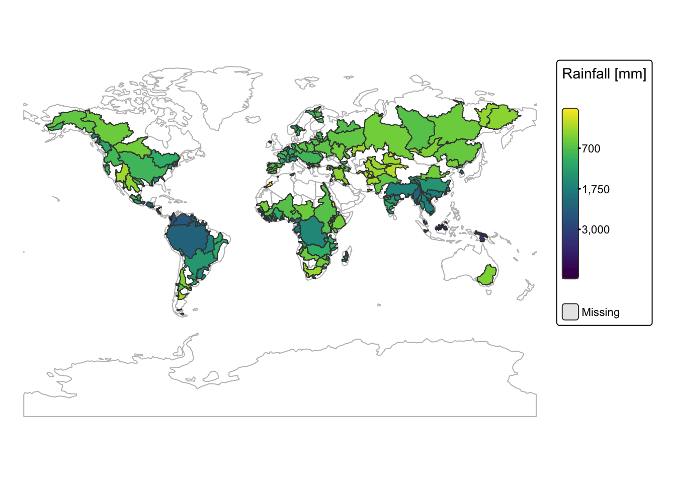
Explanation
A unique
basin_idis added to each polygon. The sf object is converted to a terraSpatVectorusingvect()for compatibility with terra functions.rasterize()creates a raster where each cell is labeled with the correspondingbasin_id, aligning with the original raster’s resolution and extent.zonal()calculates the average of raster values within each zone defined by the rasterized polygons. We then inspect and, if needed, rename the first column tozoneso that it can join withbasin_id.The zonal statistics are merged into the original basins object using a left join. The new attribute, called
precip, holds the averaged raster values for each polygon.
Geometry operations
Buffers
Buffer operations create zones around spatial features by extending
their boundaries by a specified distance. Regardless of the input
geometry (i.e., point, line, or polygon), the resulting buffers will
always be polygons. Both sf and terra
provide functions for calculating buffers: st_buffer() in
sf and buffer() in
terra.
In the following example, we use st_buffer() in
sf with the tect_plates and
ne_pop data layers to identify major cities located within
100 km of a plate margin. Plate margins are associated with increased
seismic activity, making nearby cities more vulnerable to
earthquakes.
To ensure accurate distance measurements, we first project both
layers to the Eckert IV projection, avoiding the need to
express distances in angular units (i.e., arc degrees). Since we are
only interested in major cities, we filter ne_pop before
projecting, removing all populated places with POP_MAX <
5 million.
# ESRI authority code for Eckert IV = ESRI:54012
plates_eck4 <- st_transform(tect_plates, crs = "ESRI:54012")
# Drop populated places with pop < 5 mill and then project
filtered_pop <- ne_pop %>%
filter(POP_MAX >= 5000000)
pop_eck4 <- st_transform(filtered_pop, crs = "ESRI:54012")Next, we convert plates_eck4 from
POLYGON geometry to LINE
(MULTILINESTRING) geometry, as we need buffers on both sides of the
plate margins. We then calculate the buffers and intersect them with
pop_eck4 to identify major cities within the 100 km buffer
zone.
# Convert polygons to lines by casting to MULTILINESTRING
plates_line <- st_cast(plates_eck4, "MULTILINESTRING")
# Buffer each line by 100 km = 100000 m
buffers_plates <- st_buffer(plates_line, dist = 100000)
buffers_diss <- st_union(buffers_plates) # Dissolve buffers into single geometry
# Select cities that are fully within the plate buffers
pop_within <-
pop_eck4[st_within(pop_eck4, buffers_diss, sparse = FALSE), ]
# Switch to startic mode
tmap_mode("plot")
# Plot cities as bubbles to show population
# Set bbox to plates
bbox_plates <- st_bbox(plates_eck4)
cntry_map <-
tm_shape(ne_cntry, bbox = bbox_plates) +
tm_borders("gray")
bnd_map <- cntry_map +
tm_shape(plates_eck4) +
tm_borders("black")
bnd_map +
tm_shape(pop_within) +
tm_bubbles(size = "POP_MAX",
scale=2,
col = "red",
alpha = 0.5,
title.size = "Population") +
tm_layout(frame = FALSE,
legend.text.size = 0.6,
legend.title.size = 0.6,
legend.position = c("right", "bottom"),
legend.bg.color = "white") +
tm_crs("+proj=mill")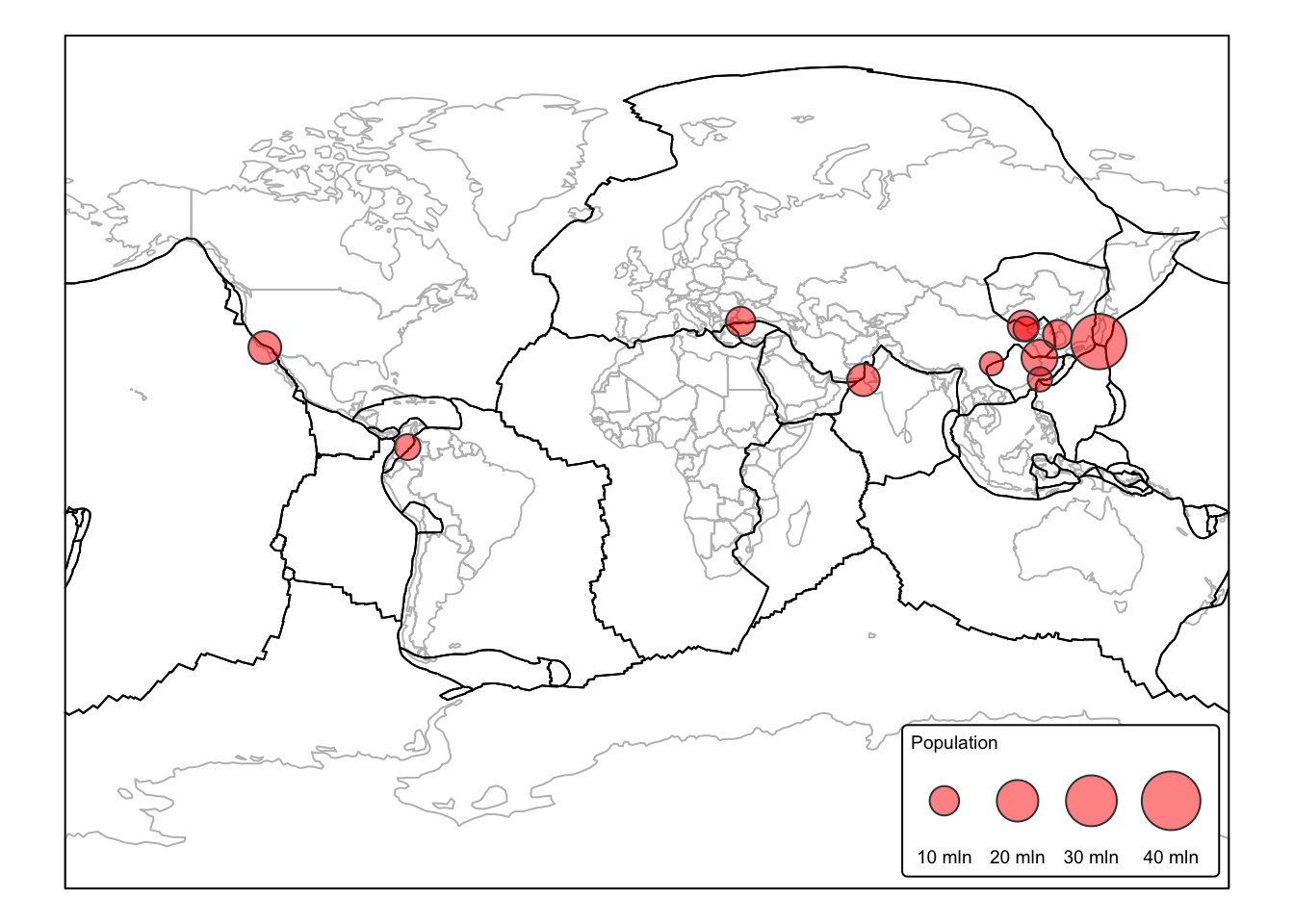
Dissolve
The dissolve operation merges adjacent or overlapping features based
on shared attributes, eliminating internal boundaries to simplify the
dataset and reveal broader spatial patterns. This process is performed
using the st_union() function in the sf
package and the aggregate() function in the
terra package.
Dissolving spatial features is often combined with spatial aggregation to compute summary statistics for specific attribute columns after merging features.
In the following example, we dissolve ne_cntry based on
the SUBREGION column and calculate the total population for
each sub-region by summing the values in the POP_EST
column.
# Use dplyr functions to dissolve
# Behind the scenes, summarize() combines the geometries and
# dissolve the boundaries between them using st_union()
ne_subregions <- ne_cntry %>%
group_by(SUBREGION) %>%
summarise(total_pop = sum(POP_EST, na.rm = TRUE))
# Switch to static mode
tmap_mode("plot")
# Plot sub-regions with colour by total_pop
tm_shape(ne_subregions) +
tm_polygons(fill = "total_pop",
fill.legend = tm_legend(title = "Sub-region \nPopulation"),
fill.scale = tm_scale_continuous_sqrt(values = "-scico.roma")) +
tm_layout(frame = FALSE) +
tm_crs("+proj=mill")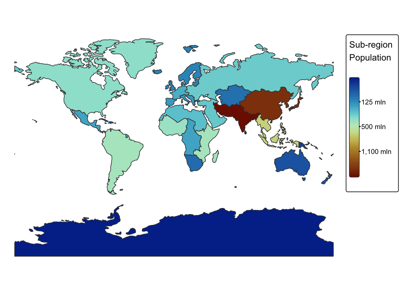
Both buffer and dissolve operations are fundamental in spatial analysis, as they help refine and interpret geographic data for various applications. Buffers are essential for proximity analysis, such as determining areas at risk from environmental hazards, planning transportation corridors, or assessing accessibility to services. Dissolve operations, on the other hand, are crucial for data simplification, thematic mapping, and statistical summarization, enabling analysts to visualize patterns at broader spatial scales.
Raster operations
Crop and Mask
The
crop()function is used to reduce a raster’s extent by selecting a subset of it. Essentially, it “crops” the raster to a smaller area defined by an extent (which can be specified as an Extent object or using the extent of another spatial object).The
mask()function applies a spatial mask to a raster. It sets the values of cells outside the mask toNA(or another specified value), effectively isolating the area of interest defined by a polygon (or another raster). The function can also perform the opposite operation: when theinverseargument is set toTRUE,mask()does the reverse — cells inside the mask becomeNAwhile retaining values outside.
In many analyses, you might use crop() first to reduce
the size of your raster to a general area and then apply
mask() to further refine that subset to a more irregular
shape.
The following example demonstrates how to use the two functions:
first, it crops the precip raster using a subset of
ne_cntry, and then it applies both a regular mask and its
inverse:
# Drop all continents excep Africa
filtered_cntry <- ne_cntry %>%
filter(CONTINENT == "Africa")
# Convert the sf object to a terra SpatVector.
africa <- vect(filtered_cntry)
# Crop the raster to the defined extent
precip_cropped <- crop(precip, africa)
names(precip_cropped) <- "precipitation"
# Apply the mask: cells outside the polygon become NA
precip_masked <- mask(precip_cropped, africa)
names(precip_masked) <- "precipitation"
# Inverse mask: masks out values **inside** the polygon
precip_mask_inverse <- mask(precip_cropped, africa, inverse = TRUE)
names(precip_mask_inverse) <- "precipitation"
# Plot precipitation rasters
rain_map1 <- tm_shape(precip_cropped) +
tm_raster("precipitation",
col.scale = tm_scale_continuous(values = "viridis"),
col.legend = tm_legend(show = FALSE)
) +
tm_layout(frame = FALSE) + tm_title("crop()", size = 1)
rain_map2 <- tm_shape(precip_masked) +
tm_raster("precipitation",
col.scale = tm_scale_continuous(values = "viridis"),
col.legend = tm_legend(show = FALSE)
) +
tm_layout(frame = FALSE) + tm_title("mask()", size = 1)
rain_map3 <- tm_shape(precip_mask_inverse) +
tm_raster("precipitation",
col.scale = tm_scale_continuous(values = "viridis"),
col.legend = tm_legend(show = FALSE)
) +
tm_layout(frame = FALSE) + tm_title("mask(inverse = TRUE)", size = 1)
tmap_arrange(rain_map1, rain_map2, rain_map3, ncol = 3)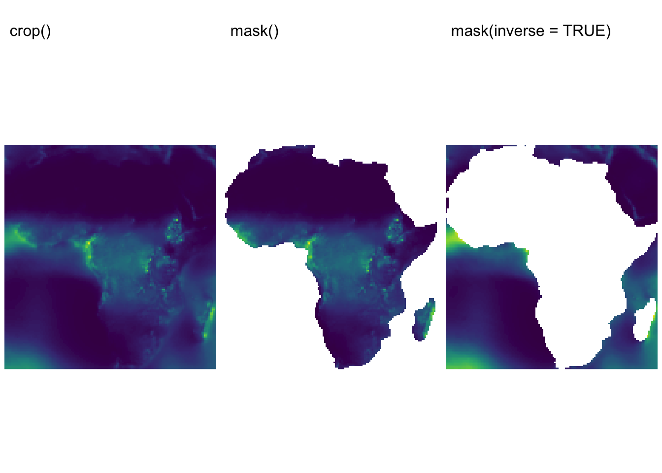
Reclassification
Reclassification of a raster generally means converting its continuous or multi-class cell values into new, often simpler, classes based on specified rules. This is useful, for instance, when you want to group values into categories (e.g., “low,” “medium”, and “high”) or to prepare data for further analysis.
In the terra package, the function
classify() is used to reclassify a raster (technically a
SpatRaster) based on a reclassification matrix. The matrix
typically has three columns:
- Column 1: Lower bound of the interval.
- Column 2: Upper bound of the interval.
- Column 3: New value or class for cells falling within that interval.
For cases where one might need more flexibility — such as applying
more complex conditional logic — one can use terra’s
ifel() function. This function works similarly to R’s base
ifelse(), but it is optimized for SpatRaster
objects.
In the next example, the continuous values in the precip
raster are grouped into five classes using defined intervals. This
approach is both efficient and clear when your classification rules are
based on ranges:
# Project raster -- for nice map
precip_proj <- project(precip,
"+proj=mill", # Output CRS
method = "bilinear", # Re-sampling method
res = 50000) # Resolution
# Define the reclassification matrix:
# - 0 to 250 becomes 1 (Arid)
# - 250 to 500 becomes 2 (Semi-arid)
# - 500 to 750 becomes 3 (Sub-humid)
# - 750 to 1000 becomes 4 (Humid)
# - >1000 becomes 5 (Very humid)
m <- matrix(c(0, 250, 1,
250, 500, 2,
500, 750, 3,
750, 1000, 4,
1000, 10000, 5),
ncol = 3, byrow = TRUE)
# Apply classification
precip_classified <- classify(precip_proj, m)
names(precip_classified) <- "precip_class"
# Plot results on map
precip_map <- tm_shape(precip_classified) +
tm_raster("precip_class",
col.scale = tm_scale_categorical(
values = c("viridis"),
labels = c("arid", "semi-arid", "sub-humid", "humid", "very humid")
),
col.legend = tm_legend(
title = "Precipitation Class",
position = tm_pos_out(cell.h = "right", cell.v = "center"),
orientation = "portrait")
) +
tm_layout(frame = FALSE,
legend.text.size = 0.6,
legend.title.size = 0.6)
# Plot countries on top
precip_map + tm_shape(ne_cntry) + tm_borders("white")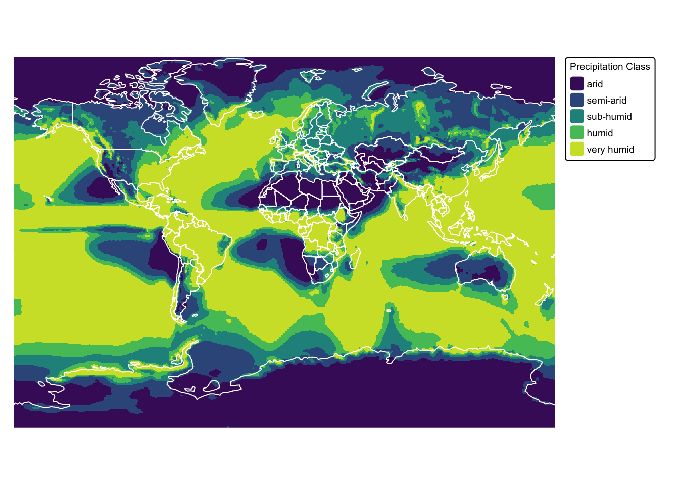
Next we illustrate the ifel() function, applying it on
the precip raster in a nested fashion to assign new values
based on the conditions specified:
# Use conditional functions to reclassify:
# - If the value is greater than 1000, assign 2.
# - Else if the value is greater than 500, assign 2.
# - Otherwise, assign NA.
precip_ifel <- ifel(precip_proj > 1000, 2, ifel(precip_proj > 500, 1, NA))
names(precip_ifel) <- "precip_class"
# Plot results on map
bbox_bnd <- st_bbox(ne_box)
precip_map <- tm_shape(precip_ifel, bbox = bbox_bnd) +
tm_raster("precip_class",
col.scale = tm_scale_categorical(
values = c("#7fcdbb", "#2c7fb8"),
labels = c("sub-humid", "humid / very humid")
),
col.legend = tm_legend(
title = "Precipitation Class",
position = tm_pos_out(cell.h = "right", cell.v = "center"),
orientation = "portrait")
) +
tm_layout(frame = FALSE,
legend.text.size = 0.6,
legend.title.size = 0.6)
# Plot countries and bnd on top
cntry_map <- precip_map + tm_shape(ne_cntry) + tm_borders("black")
cntry_map + tm_shape(ne_box) + tm_borders("black")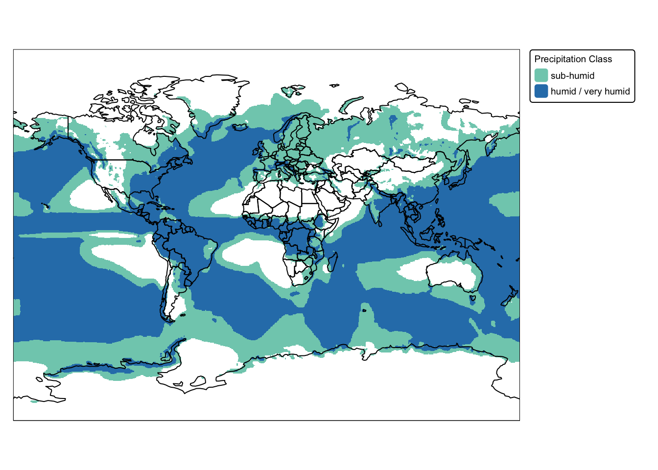
In summary, both the classify() and ifel()
functions operate on the principle of evaluating conditions to determine
an output. While classify() is often used to assign
categories or classifications based on a set of defined criteria,
ifel() typically returns one of two values depending on
whether a specific condition is met or not. Despite any differences in
naming or contextual usage, both functions essentially operate in the
same manner. Ultimately, the choice between them depends on the
complexity and structure of one’s classification rules.
Map algebra
Map algebra is a framework used in geospatial analysis to manipulate and analyze raster data through mathematical and logical operations. It involves applying arithmetic operations — like addition, subtraction, multiplication, and division — to the cell values of one or more raster layers, which allows for the creation of new datasets. It also supports conditional logic and statistical functions to transform spatial data based on defined criteria (thus, reclassification is one form of map algebra).
The following chunk of code provides several examples of map algebra
operations using the precip_proj SpatRaster:
ma1 <- precip_proj / 10 # Operation with a constant
ma2 <- sqrt(precip_proj) # Square root
ma3 <- log(precip_proj) # Base 2 log
ma4 <- ifel(precip_proj < 500, precip_proj, NA) # Conditional statement
names(ma1) <- "calc"
names(ma2) <- "calc"
names(ma3) <- "calc"
names(ma4) <- "calc"
ma_map1 <- tm_shape(ma1) +
tm_raster("calc",
col.scale = tm_scale_intervals(n = 6, values = "viridis", style = "jenks")
) +
tm_layout(frame = FALSE,
legend.text.size = 0.5,
legend.title.size = 0.5,
legend.position = c("right", "bottom"),
legend.bg.color = "white") +
tm_title("precip_proj / 10", size = 1)
ma_map2 <- tm_shape(ma2) +
tm_raster("calc",
col.scale = tm_scale_intervals(n = 6, values = "viridis", style = "jenks")
) +
tm_layout(frame = FALSE,
legend.text.size = 0.5,
legend.title.size = 0.5,
legend.position = c("right", "bottom"),
legend.bg.color = "white") +
tm_title("sqrt(precip_proj)", size = 1)
ma_map3 <- tm_shape(ma3) +
tm_raster("calc",
col.scale = tm_scale_intervals(n = 6, values = "viridis", style = "jenks")
) +
tm_layout(frame = FALSE,
legend.text.size = 0.5,
legend.title.size = 0.5,
legend.position = c("right", "bottom"),
legend.bg.color = "white") +
tm_title("log(precip_proj)", size = 1)
ma_map4 <- tm_shape(ma4) +
tm_raster("calc",
col.scale = tm_scale_intervals(n = 6, values = "viridis", style = "jenks")
) +
tm_layout(frame = FALSE,
legend.text.size = 0.5,
legend.title.size = 0.5,
legend.position = c("right", "bottom"),
legend.bg.color = "white") +
tm_title("ifel(precip_proj < 500, precip_proj, NA)", size = 1)
tmap_arrange(ma_map1, ma_map2, ma_map3, ma_map4, ncol = 2)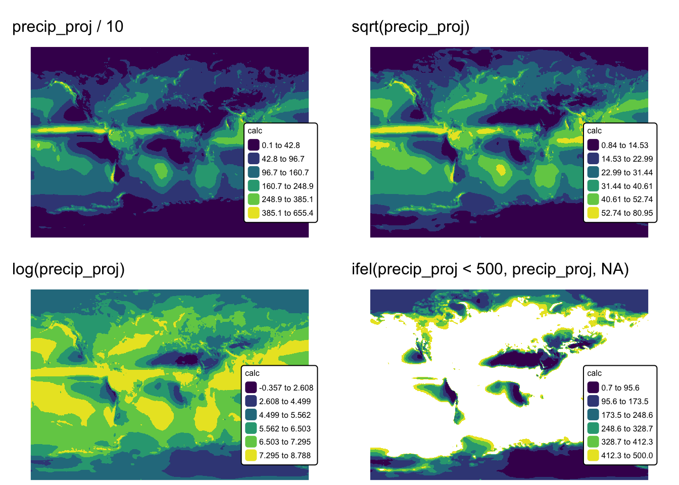
Map algebra operations can be performed on multiple rasters or between a raster and one or more non-spatial constants. When multiple rasters are involved, the mathematical or logical operation is applied to corresponding overlapping grid cells, ensuring that computations are spatially aligned. In contrast, when a raster is combined with a non-spatial constant, the operation is executed between each individual grid cell and the specified constant(s), allowing for uniform transformations across the entire dataset.
The map algebra framework underpins a variety of spatial analyses. For example, adding two raster layers that represent different environmental variables (like elevation and rainfall) can create a composite index that highlights areas of combined influence. Similarly, multiplying a raster by a constant might serve to normalize data, adjust scales, or emphasize specific features. These techniques are fundamental in tasks such as reclassification, modeling environmental phenomena, and integrating multiple datasets for comprehensive spatial analysis.
Summary
This practical provided a detailed exploration of importing and exporting geospatial data in R, including supported file formats. It also covered coordinate system transformations to ensure spatial accuracy and compatibility between datasets. Additionally, the practical introduced various geoprocessing operations for both vector and raster data.
List of R functions
This practical showcased a diverse range of R functions. A summary of these is presented below:
base R functions
aggregate(): computes summary statistics (such as mean or sum) for subsets of data defined by grouping factors. It takes a formula or a set of grouping variables and applies a function to each subset, returning a summarized data frame.attr(): is used to access or modify the attributes of an R object, such as names, dimensions, or class. It allows you to retrieve metadata stored within an object or to assign new attribute values when needed.c(): concatenates its arguments to create a vector, which is one of the most fundamental data structures in R. It is used to combine numbers, strings, and other objects into a single vector.colnames(): retrieves or sets the column names of a matrix or data frame. It simplifies the process of managing and updating the labels for columns in tabular data.data.frame(): creates a table-like structure where each column can hold different types of data. It is a primary data structure for storing and manipulating datasets in R.do.call(): calls a specified function with a list of arguments, allowing dynamic construction of function arguments. It is particularly useful when the arguments to a function are stored in a list or when programming with variable numbers of arguments.head(): returns the first few elements or rows of an object, such as a vector, matrix, or data frame. It is a convenient tool for quickly inspecting the structure and content of data.log(): calculates the logarithm of numeric values or vectors, with an option to specify the base (defaulting to the natural logarithm). It is a basic mathematical tool widely used for data transformation and analysis.matrix(): constructs a matrix by arranging a sequence of elements into specified rows and columns. It is fundamental for performing matrix computations and linear algebra operations in R.nrow(): returns the number of rows in a data frame, matrix, or other two-dimensional object. It provides a quick way to assess the size of tabular data by counting its rows.print(): outputs the value of an R object to the console. It is useful for debugging and ensuring that objects are displayed correctly within functions.runif(): generates random numbers from a uniform distribution between specified minimum and maximum values. It is commonly used in simulations or to create randomized data sets for testing and analysis.setdiff(): returns the elements present in the first vector that are not found in the second vector. It is useful for identifying unique values and comparing datasets to find non-overlapping elements.sqrt(): computes the square root for each element in a numeric vector. It is a fundamental mathematical operation that underlies many statistical and scientific computations.which(): identifies the indices of TRUE values within a logical vector. It is often used to locate positions in vectors or arrays where a given condition holds true.%in%(operator): checks for membership, returning a logical vector that indicates if elements of the left-hand vector are found within the right-hand vector. It is a handy tool for filtering, subsetting, or matching values in R.
grid functions
unit(): constructs unit objects that specify measurements for graphical parameters, such as centimeters or inches. It is often used in layout and annotation functions for precise control over plot elements.
dplyr (tidyverse) functions
%>%(pipe operator): passes the output of one function directly as the input to the next, creating a clear and readable chain of operations. It is a hallmark of the tidyverse, promoting an intuitive coding style.all_of(): selects columns from a data frame based on a character vector of column names, ensuring that all specified names exist in the data. It is especially useful in programmatic workflows within dplyr pipelines, enhancing code robustness and readability.filter(): subsets rows of a data frame based on specified logical conditions. It is essential for extracting relevant data for analysis.group_by(): organises data into groups based on one or more variables, setting the stage for group-wise operations. It is often used together with summarise or mutate.left_join(): merges two data frames by including all rows from the left data frame and matching rows from the right. It is commonly used to retain all observations from the primary dataset while incorporating additional information.select(): extracts a subset of columns from a data frame based on specified criteria. It simplifies data frames by keeping only the variables needed for analysis.summarise(): reduces multiple values down to a single summary statistic per group in a data frame. When used withgroup_by(), it facilitates the computation of aggregates such as mean, sum, or count.
ggplot2 (tidyverse) functions
aes(): defines aesthetic mappings in ggplot2 by linking data variables to visual properties such as color, size, and shape. It forms the core of ggplot2’s grammar for mapping data to visuals.ggplot(): initialises a ggplot object and establishes the framework for creating plots using the grammar of graphics. It allows for incremental addition of layers, scales, and themes to build complex visualizations.geom_boxplot(): creates box-and-whisker plots in ggplot2, summarizing data distributions through quartiles and highlighting outliers. It is a powerful tool for comparing distributions across groups.geom_errorbar(): overlays error bars on a ggplot2 plot to represent variability or uncertainty in the data. It is commonly used to display confidence intervals or standard errors alongside data points.geom_point(): adds points to a ggplot2 plot, producing scatter plots that depict the relationship between two continuous variables. It is a fundamental component for visualizing individual observations.ggtitle(): adds a main title to a ggplot2 plot, helping to contextualize the visualized data. It integrates with the overall theme of the plot to enhance interpretability and presentation.labs(): allows you to add or modify labels in a ggplot2 plot, such as titles, axis labels, and captions. It enhances the readability and interpretability of visualizations.scale_size_continuous(): maps a continuous variable to the size aesthetic of geoms in a ggplot2 plot, allowing for proportional representation of data points. It offers options to customize the range and scaling, which helps in emphasizing differences in the underlying data.xlab(): sets or modifies the label for the x-axis in a plot, providing clarity on the data dimension represented horizontally. It contributes to making plots self-explanatory by ensuring that axis information is clearly communicated.ylab(): sets or modifies the label for the y-axis in a plot, thereby improving the readability of the vertical dimension. It plays a key role in making visualizations informative by accurately describing the data plotted along the y-axis.
httr functions
build_url(): constructs a complete URL from its individual components such as scheme, hostname, path, and query parameters. It is typically used to programmatically generate URLs for API requests or web service calls.parse_url(): decomposes a URL into its constituent parts, returning a list with elements like scheme, hostname, path, and query. This function is particularly useful when you need to inspect or modify specific components of a URL.
ows4R functions
WFSClient$new(): is a constructor from the ows4R package that creates a new client object for interacting with Web Feature Services (WFS). It sets up the connection parameters, enabling users to request and retrieve spatial data from a WFS server.getFeatureTypes(): queries a WFS service to retrieve a list of available feature types or layers. This allows users to explore the data structure offered by the service and decide which layers to work with.
sf functions
st_as_sf(): converts various spatial data types, such as data frames or legacy spatial objects, into an sf object. It enables standardised spatial operations on the data.st_buffer(): creates a buffer zone around spatial features by a specified distance. It is useful for spatial analyses that require proximity searches or zone creation.st_bbox(): computes the bounding box of a spatial object, representing the minimum rectangle that encloses the geometry. It is useful for setting map extents and spatial limits.st_cast(): converts geometries from one type to another, such as from MULTIPOLYGON to POLYGON. It is helpful when a specific geometry type is required for analysis.st_collection_extract(): extracts geometries of a specified type from a geometry collection in an sf object. It is useful when you need to isolate and work with only one type of geometry (e.g., extracting only POLYGON features from a mixed geometry set).st_crs(): retrieves or sets the coordinate reference system (CRS) of spatial objects. It is essential for ensuring that spatial data align correctly on maps.st_disjoint(): tests whether geometries do not share any common points, returning a logical matrix indicating non-overlapping pairs. It is commonly used to assess spatial relationships and ensure that features do not intersect.st_join(): performs a spatial join, combining attributes from one sf object to another based on their spatial relationships (such as intersection or proximity). It is essential for integrating data from different spatial layers into a cohesive dataset.st_intersects(): checks if geometries in one sf object intersect with geometries in another, returning a logical or sparse matrix of the results. This function underpins many spatial analyses by identifying overlapping or touching features.st_polygon(): creates polygon geometries from a list of coordinate matrices, forming closed shapes. It is a core function in the sf package for constructing spatial features that represent areas.st_point(): generates point geometries from a vector of coordinates, representing specific locations in space. It is widely used for mapping individual locations or creating simple spatial objects.st_set_crs(): assigns or modifies the coordinate reference system (CRS) for an sf object. Ensuring that spatial data has the correct CRS is crucial for accurate geospatial analysis and proper alignment of layers.st_sf(): converts a regular data frame into an sf object by attaching spatial geometry information. It is the foundational step for performing spatial analysis using the simple features framework.st_transform(): reprojects spatial data into a different coordinate reference system. It ensures consistent spatial alignment across multiple datasets.st_union(): merges multiple spatial geometries into a single combined geometry. It is useful for dissolving boundaries and creating aggregate spatial features.st_within(): tests whether one set of geometries is completely contained within another set, returning a logical matrix of the containment relationship. It is useful for spatial filtering and identifying features that are fully enclosed by other features.st_write(): writes an sf object to an external file in various formats, such as shapefiles or GeoPackages. It is used to export spatial data for sharing or use in other applications.
terra functions
classify(): reclassifies the values in a raster based on a provided reclassification matrix, effectively transforming continuous data into categorical classes. This is particularly helpful for interpreting spatial patterns or for thematic mapping of raster data.crs(): retrieves or sets the coordinate reference system for spatial objects such as SpatRaster or SpatVector. It is essential for proper projection and alignment of spatial data.crop(): trims a raster to a specified spatial extent. It is used to focus analysis on a region of interest within a larger dataset.ifel(): performs element-wise conditional operations on raster data, similar to an if-else statement. It creates new rasters based on specified conditions.mask(): applies a mask to a raster using a vector or another raster, setting cells outside the desired area to NA. It is useful for isolating specific regions within a dataset.names(): gets or sets the names of layers within a SpatRaster object. It facilitates easier reference and manipulation of individual raster layers.ncell(): returns the total number of cells in a raster object, offering a quick measure of its size and resolution. It is often used to understand the extent of data or to perform validations before further processing.project(): reprojects spatial data from one CRS to another, enabling alignment of datasets. It is essential for working with spatial data from different sources.rast(): creates a new SpatRaster object or converts data into a raster format. It is the entry point for handling multi-layered spatial data in terra.rasterize(): converts vector data (such as points, lines, or polygons) into a raster format by assigning values to cells based on a specified field. This process is vital for integrating vector and raster data in spatial analyses.vect(): converts various data types into a SpatVector object for vector spatial analysis. It supports points, lines, and polygons for versatile spatial data manipulation.values(): retrieves or assigns the cell values of a SpatRaster. It allows direct manipulation of the underlying data in the raster.writeRaster(): writes a raster object to disk in various file formats, including GeoTIFF. It allows users to export processed raster data for sharing, further analysis, or use in other software environments.
tmap functions
tm_borders(): draws border lines around spatial objects on a map. It is often used in combination with fill functions to delineate regions clearly.tm_bubbles(): creates bubble maps in tmap, where the size of each bubble represents a numeric variable. It is an effective visualization tool for displaying quantitative data on spatial features with an intuitive visual metaphor.tm_dots(): plots point features on a tmap, useful for visualizing locations or events. It supports customization of size, color, and shape to enhance map interpretation.tm_fill(): fills spatial objects with color based on data values or specified aesthetics in a tmap. It is a key function for thematic mapping.tm_labels(): adds text labels to map features based on specified attributes in tmap. It is useful for annotating spatial data to improve map readability.tm_layout(): customises the overall layout of a tmap, including margins, frames, and backgrounds. It provides fine control over the visual presentation of the map.tm_legend(): customises the appearance and title of map legends in tmap. It is used to enhance the clarity and presentation of map information.tm_lines(): draws line features, such as borders or network connections, on a map. It offers customization options for line width and color to highlight spatial relationships.tm_polygons(): adds polygon layers to a tmap plot, enabling the visualization of spatial data with customizable fill colors and borders. It supports both categorical and continuous data mapping and includes options for styling legends and overall map layout.tm_pos_out(): positions map elements, such as legends or scale bars, outside the main map panel. It helps declutter the map area for a cleaner display.tm_raster(): adds a raster layer to a map with options for transparency and color palettes. It is tailored for visualizing continuous spatial data.tm_scale_continuous(): applies a continuous color scale to a raster layer in tmap. It is suitable for representing numeric data with smooth gradients.tm_scale_continuous_sqrt(): applies a square root transformation to a continuous color scale in tmap. It is useful for visualizing data with skewed distributions.tm_scale_categorical(): applies a categorical color scale to represent discrete data in tmap. It is ideal for mapping data that fall into distinct classes.tm_scale_intervals(): creates a custom interval-based color scale for a raster layer in tmap. It enhances visualization by breaking data into meaningful ranges.tm_shape(): defines the spatial object that subsequent tmap layers will reference. It establishes the base layer for building thematic maps.tm_symbols(): adds point symbols to a map with customizable shapes, sizes, and colors based on data attributes. It is useful for plotting locations with varying characteristics.tm_title(): adds a title and optional subtitle to a tmap, providing descriptive context. It helps clarify the purpose and content of the map.tmap_arrange(): arranges multiple tmap objects into a single composite layout. It is useful for side-by-side comparisons or dashboard displays.tmap_mode(): switches between static (“plot”) and interactive (“view”) mapping modes in tmap. It allows users to choose the most appropriate display format for their needs.