Runoff response of the Brisbane River catchment to the extreme rainfall of 10–11 January 2011
SCII205: Introductory Geospatial Analysis / Practical No. 9
Alexandru T. Codilean
Last modified: 2025-06-14
![]()
Introduction
In this practical, we estimate the total surface runoff generated within the Brisbane River catchment in response to the extreme rainfall event that occurred on 10–11 January 2011. Daily rainfall data from the Bureau of Meteorology (BoM) will be used to calculate the total precipitation associated with the event. A drainage network will be derived from a 250 m-resolution digital elevation model (DEM), which will then be used to route flow and compute runoff at the basin outlet.
To simplify the initial calculations, we assume that both evaporation and infiltration were negligible during the event, such that all rainfall is converted directly into surface runoff. Subsequently, we incorporate a global dataset of potential evapotranspiration to estimate the amount of evaporation that may have occurred during the event and revise our runoff calculations accordingly. The assumption of negligible infiltration is considered reasonable due to the prolonged heavy rainfall leading up to 10–11 January, which likely resulted in saturated soil conditions.
The 2010–2011 Queensland floods were among the most devastating in the state’s history, affecting approximately 75% of Queensland by January 2011. The floods highlighted the vulnerability of Queensland to natural disasters and underscored the importance of effective disaster management and mitigation strategies. In response to the disaster, a Commission of Inquiry was established to investigate the circumstances surrounding the floods and to improve future preparedness and response strategies.
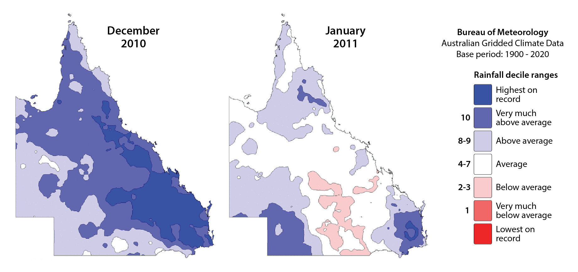
Fig. 1: Queensland rainfall deciles for Dec. 2010 and Jan. 2011.
The floods were primarily the result of prolonged heavy rainfall over the region, which was influenced by a strong La Niña event. This climatic pattern typically enhances the moisture available for rainfall, leading to unusually high and persistent rainfall amounts across south‐east Queensland (Fig. 1). The saturated catchments were then unable to absorb the successive downpours, leading to a rapid rise in river levels. Major river systems, including the Brisbane River and its tributaries, became overwhelmed.
The situation intensified when Tropical Cyclone Tasha made landfall on 25 December 2010, bringing additional heavy rains that exacerbated the flooding. On 10 and 11 January 2011, the south-east Queensland floods reached a critical and devastating phase, particularly affecting the Lockyer Valley, Ipswich, and Brisbane. These two days were marked by extreme flash flooding and widespread inundation, resulting in loss of life, severe property damage, and mass evacuations.
R packages
The practical will utilise R functions from packages explored in previous sessions:
Spatial data manipulation and analysis:
The sf package: provides a standardised framework for handling spatial vector data in R based on the simple features standard (OGC). It enables users to easily work with points, lines, and polygons by integrating robust geospatial libraries such as GDAL, GEOS, and PROJ.
The terra package: is designed for efficient spatial data analysis, with a particular emphasis on raster data processing and vector data support. As a modern successor to the raster package, it utilises improved performance through C++ implementations to manage large datasets and offers a suite of functions for data import, manipulation, and analysis.
The whitebox package: is an R frontend for WhiteboxTools, an advanced geospatial data analysis platform developed at the University of Guelph. It provides an interface for performing a wide range of GIS, remote sensing, hydrological, terrain, and LiDAR data processing operations directly from R.
Data wrangling:
- The tidyverse: is a collection of R packages designed for data science, providing a cohesive set of tools for data manipulation, visualization, and analysis. It includes core packages such as ggplot2 for visualization, dplyr for data manipulation, tidyr for data tidying, and readr for data import, all following a consistent and intuitive syntax.
Data visualisation:
- The tmap package: provides a flexible and powerful system for creating thematic maps in R, drawing on a layered grammar of graphics approach similar to that of ggplot2. It supports both static and interactive map visualizations, making it easy to tailor maps to various presentation and analysis needs.
Resources
- The Geocomputation with R book.
- The sf package documentation.
- The terra package documentation.
- The WhiteboxTools library documentation.
- The tidyverse library of packages documentation.
- The tmap package documentation.
Install and load packages
All required packages should already be installed. Should this not be the case, execute the following chunk of code:
# Main spatial packages
install.packages("sf")
install.packages("terra")

# Install the CRAN version of whitebox
install.packages("whitebox")

# For the development version run this:
# if (!require("remotes")) install.packages('remotes')
# remotes::install_github("opengeos/whiteboxR", build = FALSE)

# Install the WhiteboxTools library
whitebox::install_whitebox()

# tidyverse for additional data wrangling
install.packages("tidyverse")

# tmap dev version and leaflet for dynamic maps
install.packages("tmap",
    repos = c("https://r-tmap.r-universe.dev",
              "https://cloud.r-project.org"))
install.packages("leaflet")
Load packages:
library(sf)
library(terra)
library(tidyverse)
library(tmap)
library(leaflet)

# Set tmap to static maps
tmap_mode("plot")
Load and initialise the whitebox package:
Load and explore data
Data provided
The following datasets are provided as part of this practical exercise:
Vector data:
geofabric_river_regions.gpkg: a Geopackage containing a POLYGON geometry layer representing Australia’s Geofabric Hydrology Reporting Regions. The data layer was produced by the Bureau of Meteorology (BOM) and is part of the Australian Hydrological Geospatial Fabric (Geofabric) data product. The data layer is projected into the EPSG:3857 (WGS 84 / Pseudo-Mercator) coordinate reference system. The hydrology reporting regions generally align with Australia’s major river catchments. We will use this data layer to define a bounding box for the Brisbane River catchment.qld_pop.gpkg: a Geopackage containing a POINT geometry layer representing the location of named towns and cities in Queensland. The data was downloaded from the Queensland Government’s Spatial Catalogue, and uses a geographic coordinate systems references to the EPSG:7844 (GDA2020) datum.
Raster data:
r20110109.asctor20110112.asc: four ESRI ASCII grid files representing daily precipitation in mm for 9, 10, 11, and 12 January 2011. Although the extreme rainfall event occurred on 10-11 January, we extended our analysis to include the day before and the day after, ensuring that no rainfall was overlooked. The data was obtained from the Bureau of Meteorology (BOM). It has a spatial resolution of 0.05 degrees (approx. 5 km), and uses a geographic coordinate system referenced to the EPSG:4283 (GDA94) datum. The data is part of BOM’s Australian Gridded Climate Data (AGCD) data product, and can be downloaded from here.geodata_dem_9s.tif: a GeoTIFF file representing the GEODATA 9 Second Digital Elevation Model (DEM-9S) Version 3 from Geoscience Australia. The dataset has a resolution of 9 arc seconds (approx. 250 m) and uses a geographic coordinate system referenced to the EPSG:4283 (GDA94) datum.et0_v3_01.tif: a GeoTIFF file representing global reference evapotranspiration (PET) values in mm for the month of January calculated using monthly average climate data for the period 1970 to 2000. The data was produced by the Consortium for Spatial Information (CGIAR-CSI) and can be downloaded from here. It has a spatial resolution of 30 arc seconds (approx. 1 km), and uses a geographic coordinate system referenced to the EPSG:4326 (WGS 84) datum.
Prepare vector data
The following block of R code reads in the
geofabric_river_regions.gpkg and qld_pop.gpkg
vector layers as sf objects.
# Specify the path to the data
geofabric_file <- "./data/data_flood/vector/geofabric_river_regions.gpkg"
cities_file <- "./data/data_flood/vector/qld_pop.gpkg"

# Read in the geopackage files as sf objects using st_read()
geofabric_regions <- st_read(geofabric_file)
## Reading layer `RiverRegionWebM' from data source
## `/Volumes/Work/Dropbox/Transfer/SCII206/R-Resource/data/data_flood/vector/geofabric_river_regions.gpkg'
## using driver `GPKG'## Simple feature collection with 219 features and 17 fields
## Geometry type: MULTIPOLYGON
## Dimension: XY
## Bounding box: xmin: 12579120 ymin: -5444036 xmax: 17103020 ymax: -1120631
## Projected CRS: WGS 84 / Pseudo-Mercator## Reading layer `Population_centres' from data source
## `/Volumes/Work/Dropbox/Transfer/SCII206/R-Resource/data/data_flood/vector/qld_pop.gpkg'
## using driver `GPKG'## Simple feature collection with 740 features and 19 fields
## Geometry type: POINT
## Dimension: XY
## Bounding box: xmin: 138.1202 ymin: -28.99664 xmax: 153.5315 ymax: -9.230423
## Geodetic CRS: GDA2020## [1] "hydroid" "division" "rivregname" "srcfcname" "srcftype"
## [6] "srctype" "sourceid" "featrel" "fsource" "attrrel"
## [11] "attrsource" "planacc" "symbol" "textnote" "globalid"
## [16] "rivregnum" "albersarea" "SHAPE"## [1] "feature_type" "name" "alternate_name"
## [4] "qld_pndb_id" "attribute_source" "attribute_date"
## [7] "additional_names" "add_names_source" "feature_source"
## [10] "feature_date" "operational_status" "population"
## [13] "population_date" "local_government" "pfi"
## [16] "ufi" "upper_scale" "text_note"
## [19] "add_information" "Shape"The geofabric_regions sf object
includes an attribute column named rivregname that
stores the names of the various GEOFABRIC river regions. The subsequent
block of R code extracts the Brisbane River catchment from
geofabric_regions by filtering on
rivregname.
# Filter geofabric_regions
brisbane_catchment <- geofabric_regions %>%
  filter(rivregname == "BRISBANE RIVER")
Next, we project brisbane_catchment and
qld_pop to EPSG:3577 (GDA94 / Australian Albers) and create
a 10 km buffer around the Brisbane River catchment to be used for
cropping and masking qld_pop and the raster data.
# Project to EPSG:3577
brisbane_catchment_proj <- st_transform(brisbane_catchment, crs = "EPSG:3577")
qld_pop_proj <- st_transform(qld_pop, crs = "EPSG:3577")

# Create 10km buffer
bris_buff <- st_buffer(brisbane_catchment_proj, dist = 10000)
bris_buff_diss <- st_union(bris_buff) # Dissolve buffers into single geometry
Filter qld_pop_proj to drop all populated places that
are located outside of the Brisbane River 10 km buffer:
# Extract all populated places within the 10 km buffer
brisbane_cities_proj <-
  qld_pop_proj[apply(st_intersects(qld_pop_proj, bris_buff_diss, sparse = FALSE), 1, any), ]
Plot all vector layers on an interactive map using tmap:
# Set tmap to view mode (for interactive maps)
tmap_mode("view")

# Create a tmap layer for the catchment boundaries
map_catchment <- tm_shape(brisbane_catchment_proj) +
  tm_borders("darkred") +
  tm_fill("red", fill_alpha = 0.2) +
  tm_shape(bris_buff_diss) + # Add buffers
     tm_borders("black",  lty = "dashed")

# Create a tmap layer for cities with symbols and labels
map_cities <- tm_shape(brisbane_cities_proj) +
        tm_symbols(shape = 22, size = 0.6, fill = "white") +
        tm_labels("name", size = 0.8, col = "black", xmod = unit(0.1, "mm"))

# Combine all layers to create the final map
map_catchment + map_cities
Prepare raster data
The following block of R code loads the BOM precipitation rasters,
reprojects them to EPSG:3577 (GDA94 / Australian Albers), and then crops
them to the extent of bris_buff_diss.
# Define BOM file paths in a vector
bom_files <- c(
  "./data/data_flood/raster/r20110109.asc",
  "./data/data_flood/raster/r20110110.asc",
  "./data/data_flood/raster/r20110111.asc",
  "./data/data_flood/raster/r20110112.asc"
)

# Define source and target CRS and resampling parameters
source_crs <- "EPSG:4283"
target_crs <- "EPSG:3577"
res_val_rain <- 5000

# Initialise a list to store the reprojected BOM rasters
proj_rasters <- list()

# Loop over each BOM file using an index
for (i in seq_along(bom_files)) {
  file <- bom_files[i]
  # Read the raster
  r <- rast(file)
  # Assign the source CRS
  crs(r) <- source_crs
  # Reproject the raster
  r_proj <- project(r, target_crs, method = "bilinear", res = res_val_rain)
  # Store the reprojected raster in the list
  proj_rasters[[i]] <- r_proj
}

# Combine the individual BOM rasters into a SpatRaster stack
bom_stack <- rast(proj_rasters)

# Crop and mask to extent of bris_buff_diss sf object
# Convert to a terra SpatVector
bnd_mask <- vect(bris_buff_diss)

# Crop BOM stack
bom_stack <- crop(bom_stack, bnd_mask)
Plot daily rainfall rasters using tmap:
# Define elements and their full names
layer_names <- c("20110109", "20110110", "20110111", "20110112")

facet_date <- c(`20110109` = "09 Jan.",
                `20110110` = "10 Jan.",
                `20110111` = "11 Jan.",
                `20110112` = "12 Jan."
               )

# Set the names for each layer to be used as facet labels.
names(bom_stack) <- paste0(facet_date[layer_names])

# Set tmap to static mode
tmap_mode("plot")

# Create faceted map of daily rainfall
tm_shape(bom_stack) +
  tm_raster(col.scale = tm_scale_continuous(values = "-scico.oslo", n = 4),
            col.legend = tm_legend(title = "Rainfall \n[mm]",
                                   position = tm_pos_out("right", "center")),
            col.free = FALSE) +  # Add one common legend
tm_shape(brisbane_catchment_proj) + tm_borders("darkred") + # Add a tmap layer for catchment
tm_layout(frame = TRUE,
          legend.text.size = 0.7,
          legend.title.size = 0.7,
          legend.position = c("right", "bottom"),
          legend.bg.color = "white",
          panel.label.bg.color = 'linen') +
  tm_facets(ncol = 4, free.scales = FALSE) # Plot each raster as a facet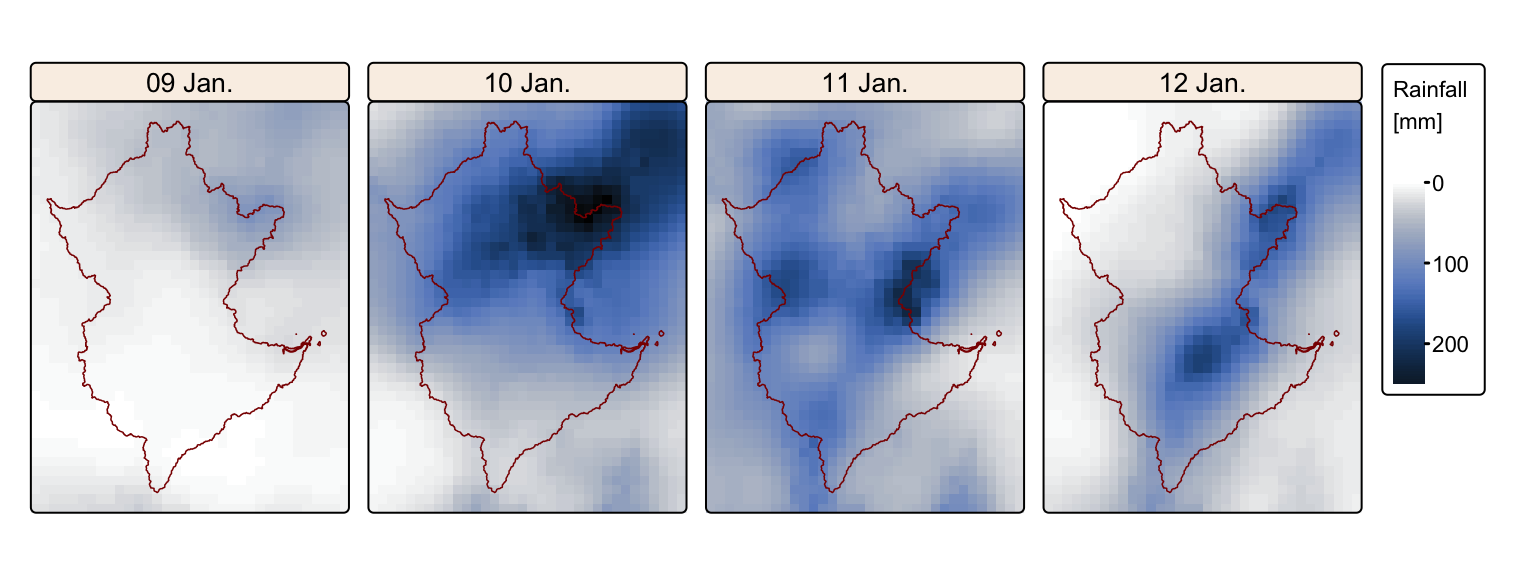
The maps confirm the high rainfall totals recorded on 10 and 11 January. Although rainfall on 9 January was negligible, significant rainfall also occurred on 12 January. Therefore, for the purposes of subsequent analyses, we will consider total rainfall over the period 9–12 January, rather than limiting the analysis to only 10 and 11 January.
The next block of R code loads the DEM and PET rasters, reprojects
them to EPSG:3577 (GDA94 / Australian Albers), and then crops and masks
them to the extent of bris_buff_diss.
# Path to files
geodata_dem <- "./data/data_flood/raster/geodata_dem_9s.tif"
pet_raster <- "./data/data_flood/raster/et0_v3_01.tif"

dem <- rast(geodata_dem)
dem_proj <- project(dem, target_crs, method = "bilinear", res = 250)
names(dem_proj) <- "Elevation"

pet <- rast(pet_raster)
pet_proj <- project(pet, target_crs, method = "bilinear", res = 1000)
## |---------|---------|---------|---------|## ==============## =============## ============== names(dem_proj) <- "PET"
# Crop and mask DEM
# Mask: cells outside the polygon become NA
dem_proj <- crop(dem_proj, bnd_mask)
dem_proj_mask <- mask(dem_proj, bnd_mask)
names(dem_proj_mask) <- "Elevation"
# Crop PET (we will mask later)
pet_proj <- crop(pet_proj, bnd_mask)Sum rainfall values and resample all rasters to match DEM extent and resolution:
# Sum rainfall rasters
rain_tot <- sum(bom_stack)

# Resample to match DEM
rain_250m <-resample(rain_tot, dem_proj_mask, method = "bilinear")
rain_250m <- mask(rain_250m, bnd_mask)
names(rain_250m) <- "Rainfall"

pet_250m <-resample(pet_proj, dem_proj_mask, method = "bilinear")
pet_250m <- mask(pet_250m, bnd_mask)

# Calculate daily PET
pet_250m_day <- pet_250m / 31
names(pet_250m_day) <- "PET"
Plot final rasters on a map:
# Set tmap to static maps
tmap_mode("plot")

# Plot rainfall on map
map1 <- tm_shape(rain_250m) +
    tm_raster("Rainfall",
        col.scale = tm_scale_intervals(values = "-scico.oslo", n=6, style = "fisher"),
        col.legend = tm_legend(title = "Rainfall [mm]")) +
    tm_layout(frame = FALSE,
          legend.text.size = 0.7,
          legend.title.size = 0.7,
          legend.position = c("right", "bottom"),
          legend.bg.color = "white") +
tm_shape(brisbane_catchment_proj) + tm_borders("darkred") + # Add a tmap layer for catchment
tm_scalebar(position = c("left", "top"), width = 10) # Add scalebar

# Plot PET on map
map2 <- tm_shape(pet_250m_day) +
    tm_raster("PET",
        col.scale = tm_scale_intervals(values = "-scico.nuuk", n=6, style = "fisher"),
        col.legend = tm_legend(title = "PET [mm/day]")) +
    tm_layout(frame = FALSE,
          legend.text.size = 0.7,
          legend.title.size = 0.7,
          legend.position = c("right", "bottom"),
          legend.bg.color = "white") +
tm_shape(brisbane_catchment_proj) + tm_borders("darkred") + # Add a tmap layer for catchment
tm_scalebar(position = c("left", "top"), width = 10) # Add scalebar

# Plot dem on map
map3 <- tm_shape(dem_proj_mask) +
    tm_raster("Elevation",
        col.scale = tm_scale_intervals(values = "hcl.terrain2", n=6, style = "fisher"),
        col.legend = tm_legend(title = "Elevation [m a.s.l.]")) +
    tm_layout(frame = FALSE,
          legend.text.size = 0.7,
          legend.title.size = 0.7,
          legend.position = c("right", "bottom"),
          legend.bg.color = "white") +
tm_shape(brisbane_catchment_proj) + tm_borders("darkred") + # Add a tmap layer for catchment
tm_scalebar(position = c("left", "top"), width = 10) # Add scalebar

tmap_arrange(map1,map2,map3)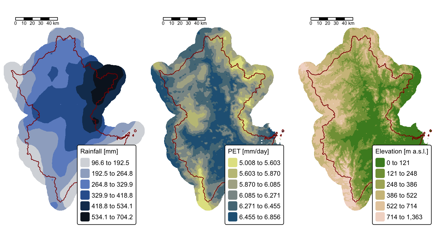
The above maps illustrate the three rasters that will be used to estimate surface runoff in the Brisbane River catchment resulting from the 10-11 January event.
Before proceeding with the runoff calculations, it is necessary to delineate the actual watershed of the Brisbane River, excluding all areas upstream of the Wivenhoe Dam. Although water was released from the Wivenhoe reservoir following the rainfall event — contributing to the peak in the Brisbane River on 13 January — runoff from areas upstream of the dam did not contribute to surface flow during the 10–11 January event. Therefore, these upstream areas will be excluded from the runoff analysis.
Watershed mapping and analysis
Watershed delineation in terrain analysis involves using a DEM to identify and outline the area, or catchment, that contributes surface runoff to a specific point (often called the pour point). This process is fundamental for hydrological modelling, water resource management, and environmental planning.
Below is an overview of the key steps involved:
DEM preprocessing: the DEM is first preprocessed to remove artefacts and fill depressions (or sinks) that might disrupt the natural flow of water (Fig. 2). This “sink-filling” step ensures a continuous and hydrologically sound surface.
Flow direction calculation: algorithms such as the D8 method (Fig. 2) are used to determine the direction of flow from each cell in the DEM, typically directing flow to the neighbouring cell with the steepest descent. This step establishes the primary flow paths across the terrain.
Flow accumulation: once flow directions are set, each cell’s flow accumulation is computed by counting the number of upstream cells that contribute runoff to it. Cells with high accumulation values typically represent stream channels.
Stream network extraction: a threshold is applied to the flow accumulation grid to extract the stream network. This network serves as a framework for identifying the main channels and tributaries within the watershed.
Watershed boundary delineation: starting from a defined pour point (often located at the outlet of a stream), the watershed boundary is delineated by tracing all cells that drain into that point. This aggregation of contributing cells forms the watershed.
The flow direction raster is a cornerstone of hydrological modelling in geospatial analysis, providing a basis for extracting stream networks, delineating watersheds, and calculating metrics such as the length of flow paths both upstream and downstream. Several well-established algorithms exist to compute flow direction, each with its own characteristics, strengths, and limitations. The main ones include (Fig. 2):
D8 (deterministic 8-neighbour) algorithm: this classic method directs flow from each cell to its steepest descending neighbour among the eight surrounding cells. It is computationally efficient but may oversimplify flow patterns in complex or flat terrains.
D-infinity (Dinf) algorithm: this approach computes flow direction as a continuous variable, allowing the assignment of flow along any downslope angle between cell centres. It offers improved representation of convergent and divergent flows in intricate landscapes.
Multiple flow direction (MFD) algorithm: unlike the D8 method, MFD methods such as FD8 distribute flow across all downslope neighbours rather than a single cell. This can provide a more realistic simulation of water dispersion, particularly in areas with gently sloping or ambiguous drainage paths.
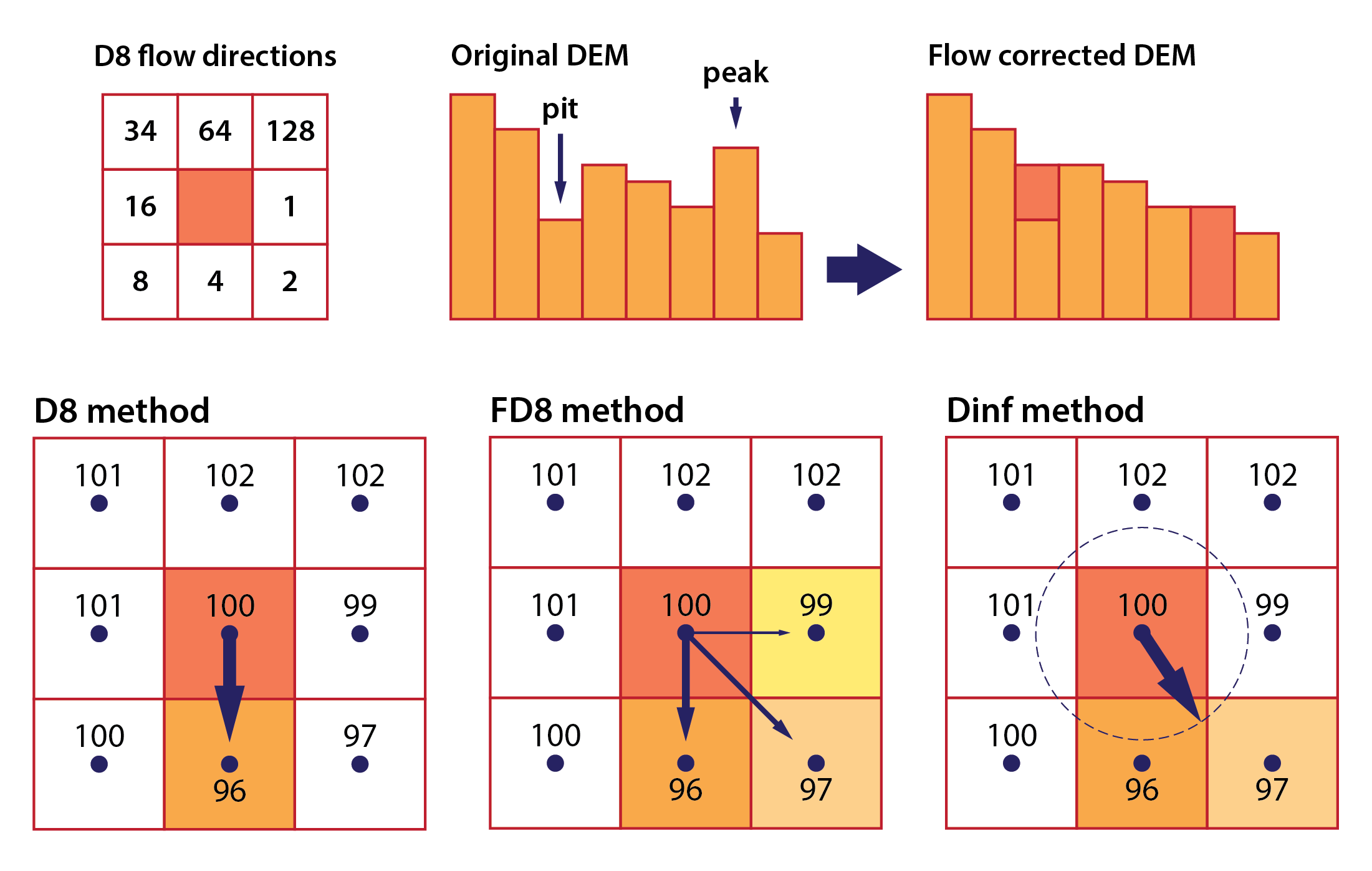
Fig. 2: D8 flow directions are coded with integers representing powers of 2 (top left), the principles behind DEM flow conditioning (top right), and the apportionment of flow directions in the D8, FD8, and Dinf flow routing methods (bottom).
Save rasters to disk
We will use the hydrological analysis functions provided by the WhiteboxTools library — accessed via the whitebox R package — to delineate the Brisbane River watershed and compute surface runoff. The whitebox package requires raster datasets to be read from disk rather than operated on as in-memory objects. While this design choice may appear inconvenient, it enables the efficient processing of large datasets that might otherwise exceed available system memory.
The following block of R code writes dem_proj_mask to
disk in GeoTIFF format:
Compute flow grid
Remove depressions from DEM
WhiteboxTools offers a couple of approaches for handling
depressions in DEMs, each designed to ensure continuous flow paths for
hydrological analysis while minimising the alteration of the original
terrain. The wbt_fill_depressions() function fills
depressions in a DEM by raising cell elevations to the lowest spill
point, ensuring a continuous drainage network while minimising large
flat areas. Alternatively, wbt_breach_depressions() and
wbt.breach_depressions_least_cost() preserve topographic
detail by lowering barrier cells to create outflow channels, with the
latter using a least-cost algorithm to minimise terrain alteration.
While the least-cost method offers the most terrain-preserving approach, full depression filling remains useful in certain contexts, and both can be combined for improved results. The following block of R code generates a hydrologically continuous DEM by both breaching and filling depressions.
# Specify input raster
qld_dem <- "./data/dump/flood/qld_dem250m.tif"

# Specify output rasters
qld_breached_dem <- "./data/dump/flood/qld_breached_250m.tif"
qld_filled_dem <- "./data/dump/flood/qld_filled_250m.tif"

# Breach depressions
# Options:
# dist - maximum search distance for breach paths in cells
# max_cost - optional maximum breach cost (default is Inf)
# min_dist - optional flag indicating whether to minimize breach distances
# flat_increment - optional elevation increment applied to flat areas
# fill - optional flag indicating whether to fill any remaining unbreached depressions
wbt_breach_depressions_least_cost(
            dem = qld_dem,
            output = qld_breached_dem,
            dist = 1000
          )

# Fill depressions
# Options:
# fix_flats - optional flag indicating if flat areas should have a small gradient applied
# flat_increment - optional elevation increment applied to flat areas
# max_depth - optional maximum depression depth to fill
wbt_fill_depressions(
            dem = qld_breached_dem,
            output = qld_filled_dem,
            fix_flats=TRUE
          )
Calculate D8 flow direction
WhiteboxTools includes several algorithms for calculating flow direction from a DEM, including the D8, FD8, and Dinf methods described above. Below we use the D8 method as this is a requirement for stream network extraction and watershed delineation:
Calculate D8 flow accumulation
As with flow direction above, WhiteboxTools includes several algorithms for calculating flow accumulation, including the D8, FD8, and Dinf methods. Once again we use the D8 method:
# Specify output raster
qld_flow <- "./data/dump/flood/qld_d8flow.tif"

# D8 Options:
# out_type - output type; one of 'cells' , 'catchment area', 'specific contributing area'
# log - optional flag to request the output be log-transformed
# clip - optional flag to request clipping the display max by 1%
# pntr - is the input raster a D8 flow pointer rather than a DEM?
# esri_pntr - input D8 pointer uses the ESRI style scheme
wbt_d8_flow_accumulation(
             i = qld_flowdir,
             output = qld_flow,
             out_type = "cells",
             pntr = TRUE,
             esri_pntr=TRUE
           )
Extract stream network
The next block of R code extracts a stream network from
qld_dem and orders the streams according to the Strahler
stream ordering scheme.
The function wbt_extract_streams() requires a flow
accumulation grid calculated using the D8 flow routing
method and a threshold basin area value, which represents the area at
which flow transitions from a diffusive to an advective regime, leading
to the formation of streams. A commonly used threshold value is 1 square
kilometre, based on empirical evidence from hydrological and
geomorphological studies that identify this scale as a typical point
where channelisation begins in many landscapes.
# Specify paths to output stream rasters
qld_streams <- "./data/dump/flood/qld_stream.tif"
qld_strahler <- "./data/dump/flood/qld_strahler.tif"

# Extract streams
# Here we chose a threshold of 16 pixels = 1km2 (250m DEM)
wbt_extract_streams(
    flow_accum = qld_flow,      # D8 flow accumulation file
    output = qld_streams,       # Output raster file
    threshold = 16,             # Threshold in flow accumulation for channelization
    zero_background=FALSE       # Use NoData for no streams
)

# Do Strahler stream ordering
wbt_strahler_stream_order(
    d8_pntr = qld_flowdir,      # D8 pointer raster file,
    streams = qld_streams,      # Raster streams file
    output = qld_strahler,      # Output Strahler raster
    esri_pntr=TRUE,             # D8 pointer uses the ESRI style scheme
    zero_background=FALSE       # Use NoData for no streams
)
Plot the Strahler network along with
brisbane_cities_proj on an interactive map:
# Load Strahler raster

strahler <- rast(qld_strahler)
names(strahler) <- "Strahler No."

# Set tmap to view mode (for interactive maps)
tmap_mode("view")

# Create a tmap layer for the catchment boundaries
map_strahler <- tm_shape(strahler) +
  tm_raster("Strahler No.", col.scale = tm_scale_categorical(values = "-scico.managua")) +
  tm_shape(bris_buff_diss) + # Add buffers
     tm_borders("black",  lty = "dashed")

# Create a tmap layer for cities with symbols and labels
map_cities <- tm_shape(brisbane_cities_proj) +
        tm_symbols(shape = 22, size = 0.6, fill = "white")

# Combine all layers to create the final map
map_strahler + map_cities
Delineate watersheds
In the next step, our objective is to delineate two watersheds: one representing the area draining through the city of Brisbane, and the other representing the area upstream of the Wivenhoe Dam.
Watershed delineation is performed using the
Watershed tool, which is invoked through the
WhiteboxTools wtb_watershed() function. This
function requires a D8 flow direction raster and a pour
point file in ESRI shapefile format.
We will generate the pour point file using the locations of two
population centres: the city of Brisbane (taken from
brisbane_cities_proj), and Wivenhoe Pocket, which is
situated on the Brisbane River just downstream of the Wivenhoe Dam. To
ensure the pour points align with the extracted stream network, we will
use the WhiteboxTools
wbt_jenson_snap_pour_points() function to snap them to the
nearest stream cell. To further ensure that the pour points snap to the
appropriate stream cells, we filter the stream network raster by
removing all cells with a Strahler stream order less than 6 (see
interactive map above).
# Extract Brisbane from 'brisbane_cities_proj'
brisbane_coords <- brisbane_cities_proj %>%
  filter(name == "Brisbane") %>%
  st_coordinates()

# Extract coordinates for Brisbane
brisbane_x <- brisbane_coords[1, 1]
brisbane_y <- brisbane_coords[1, 2]

# Define Wivenhoe Pocket coordinates manually (WGS84, then transform)
wivenhoe_coords <- st_sfc(
  st_point(c(152.6125, -27.4041)),  # lon, lat in WGS84
  crs = 4326
) %>%
  st_transform(crs = 3577)

# Create combined sf object with both points
pour_points <- st_sf(
  pop = c("Wivenhoe Pocket", "Brisbane"),
  geometry = st_sfc(
    wivenhoe_coords[[1]],
    st_point(c(brisbane_x, brisbane_y))
  ),
  crs = 3577
)

# Write pour points file to disk
st_write(pour_points, "./data/dump/flood/qld_ppoints_raw.shp", delete_dsn = TRUE)
## Deleting source `./data/dump/flood/qld_ppoints_raw.shp' using driver `ESRI Shapefile'
## Writing layer `qld_ppoints_raw' to data source
## `./data/dump/flood/qld_ppoints_raw.shp' using driver `ESRI Shapefile'
## Writing 2 features with 1 fields and geometry type Point.# Filter stream network raster to only include values with Strahler n < 6
stream_network <- rast(qld_streams)
strahler_ifel <- ifel(strahler < 6, NA, stream_network)
writeRaster(strahler_ifel, "./data/dump/flood/qld_stream_s6.tif", overwrite = TRUE)
# Path to files
brisbane_pourpoints_raw <- "./data/dump/flood/qld_ppoints_raw.shp"
brisbane_pourpoints_snapped <- "./data/dump/flood/qld_ppoints_snapped.shp"
brisbane_streams <- "./data/dump/flood/qld_stream_s6.tif"
# Snap pour points
wbt_jenson_snap_pour_points(
pour_pts = brisbane_pourpoints_raw,
streams = brisbane_streams,
output = brisbane_pourpoints_snapped,
snap_dist = 20000 # Maximum snap distance in map units
)
# Specify paths to output watershed raster
qld_bas <- "./data/dump/flood/qld_wtsheds.tif"
# Delineate watersheds
wbt_watershed(
d8_pntr = qld_flowdir, # D8 pointer raster file
pour_pts = brisbane_pourpoints_snapped, # Pour points (outlet) file
output = qld_bas, # Output raster file
esri_pntr=TRUE # D8 pointer uses the ESRI style scheme
)
# Read in watershed raster
brisbane_basins <- rast(qld_bas)
names(brisbane_basins) <- "Basin ID"Plot watersheds and stream network on a map:
# Set tmap to static maps
tmap_mode("plot")

# Plot watersheds and stream network
tm_shape(brisbane_basins) +
  tm_raster("Basin ID",
        col.scale = tm_scale_categorical(values = c("linen", "lavenderblush")),
        col.legend = tm_legend(title = "Basin ID")) +
tm_shape(strahler) +
  tm_raster("Strahler No.", col.scale = tm_scale_categorical(values = "-scico.oslo")) +
tm_layout(frame = FALSE,
      legend.text.size = 0.7,
      legend.title.size = 0.7,
      legend.bg.color = "white") +
tm_scalebar(position = c("left", "top"), width = 10) # Add scalebar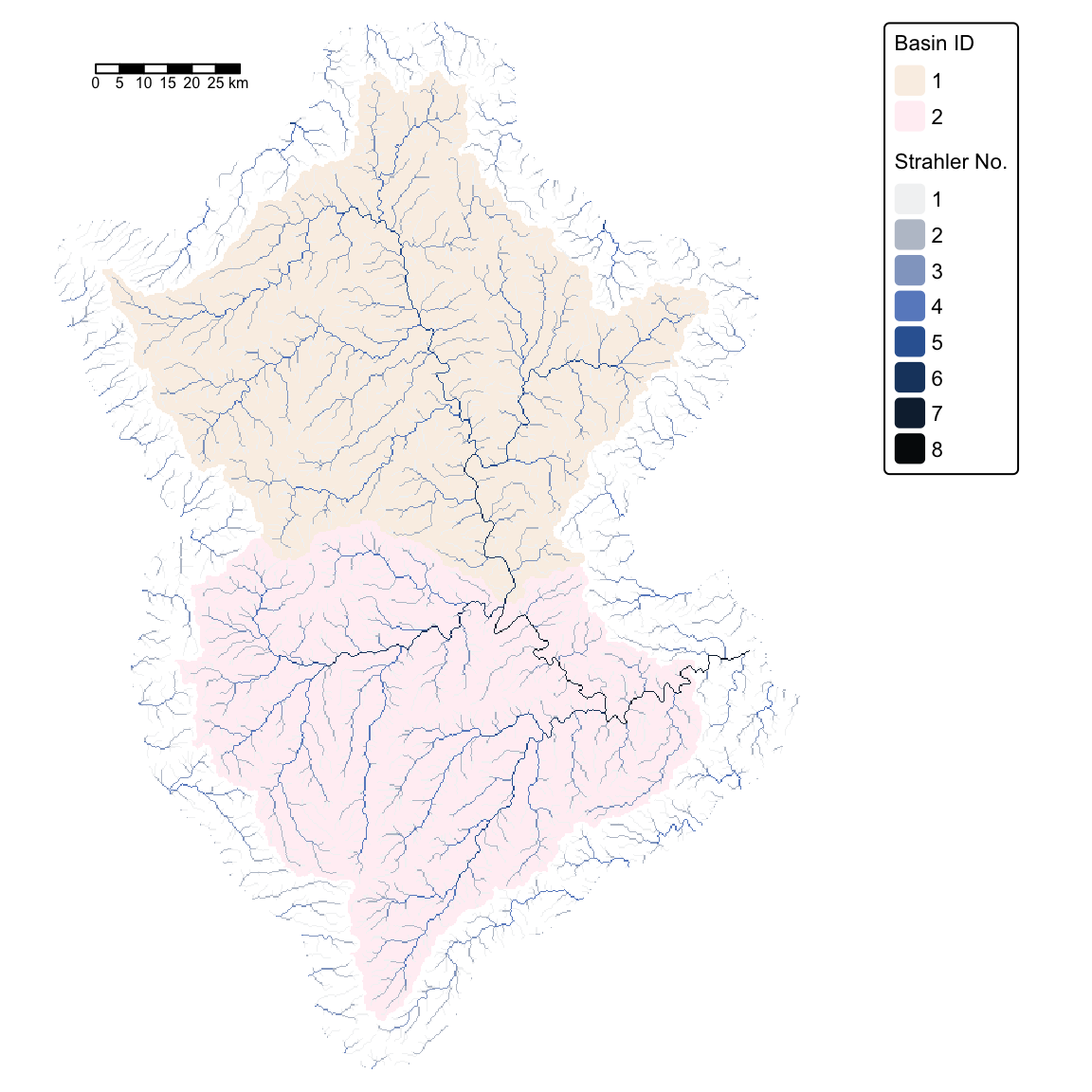
We now have all the required data layers to calculate the total surface runoff at the outlet of the Brisbane River, excluding contributions from areas upstream of the Wivenhoe Dam.
Estimate total surface runoff
Remove Wivenhoe watershed
The following block of code filters the brisbane_basins
raster to remove the areas upstream of the Wivenhoe Dam. The filtered
raster is then used to crop and mask the DEM, and rainfall and PET
rasters prior to the runoff calculations.
# Reclassify 'brisbane_basins' so that areas upstream of
# Wivenhoe Dam is set to null
brisbane_rast <- ifel(brisbane_basins == 1, NA, 1)
names(brisbane_rast) <- "BasinID"

# Convert to polygons
brisbane_mask <- as.polygons(brisbane_rast)
# Optionally remove NA polygons
brisbane_mask <- brisbane_mask[!is.na(brisbane_mask$BasinID), ]

# Read in filled DEM and crop and mask
filled_dem <- rast(qld_filled_dem)
brisbane_dem <- crop(filled_dem, brisbane_mask)
brisbane_dem <- mask(brisbane_dem, brisbane_mask)
names(brisbane_dem) <- "Elevation"

# Crop and mask the rainfall and PET rasters
# Rainfall
rain_bris <- crop(rain_250m, brisbane_mask)
rain_bris <- mask(rain_bris, brisbane_mask)
names(rain_bris) <- "Rainfall"
# PET
pet_bris_day <- crop(pet_250m_day, brisbane_mask)
pet_bris_day <- mask(pet_bris_day, brisbane_mask)
names(pet_bris_day) <- "PET"

# PET for 4 days (9 - 12 Jan)
pet_total <- pet_bris_day * 4

# Remove no data values and mask again
pet_total[is.na(pet_total)] <- 1
pet_total <- mask(pet_total, brisbane_mask)

# Save cropped and masked rasters to disk
writeRaster(brisbane_dem, "./data/dump/flood/qld_dem_brisbane.tif", overwrite = TRUE)
writeRaster(pet_total, "./data/dump/flood/qld_pet250m.tif", overwrite = TRUE)
writeRaster(rain_bris, "./data/dump/flood/qld_rain250m.tif", overwrite = TRUE)
Plot the cropped rasterst on a map:
# Set tmap to static maps
tmap_mode("plot")

# Plot rainfall on map
map1 <- tm_shape(rain_bris) +
    tm_raster("Rainfall",
        col.scale = tm_scale_intervals(values = "-scico.oslo", n=6, style = "fisher"),
        col.legend = tm_legend(title = "Rainfall [mm]")) +
    tm_layout(frame = FALSE,
          legend.text.size = 0.7,
          legend.title.size = 0.7,
          legend.position = c("right", "bottom"),
          legend.bg.color = "white") +
tm_scalebar(position = c("left", "top"), width = 10) # Add scalebar

# Plot PET on map
map2 <- tm_shape(pet_bris_day) +
    tm_raster("PET",
        col.scale = tm_scale_intervals(values = "-scico.nuuk", n=6, style = "fisher"),
        col.legend = tm_legend(title = "PET [mm/day]")) +
    tm_layout(frame = FALSE,
          legend.text.size = 0.7,
          legend.title.size = 0.7,
          legend.position = c("right", "bottom"),
          legend.bg.color = "white") +
tm_scalebar(position = c("left", "top"), width = 10) # Add scalebar

# Plot dem on map
map3 <- tm_shape(brisbane_dem) +
    tm_raster("Elevation",
        col.scale = tm_scale_intervals(values = "hcl.terrain2", n=6, style = "fisher"),
        col.legend = tm_legend(title = "Elevation [m a.s.l.]")) +
    tm_layout(frame = FALSE,
          legend.text.size = 0.7,
          legend.title.size = 0.7,
          legend.position = c("right", "bottom"),
          legend.bg.color = "white") +
tm_scalebar(position = c("left", "top"), width = 10) # Add scalebar

tmap_arrange(map1,map2,map3)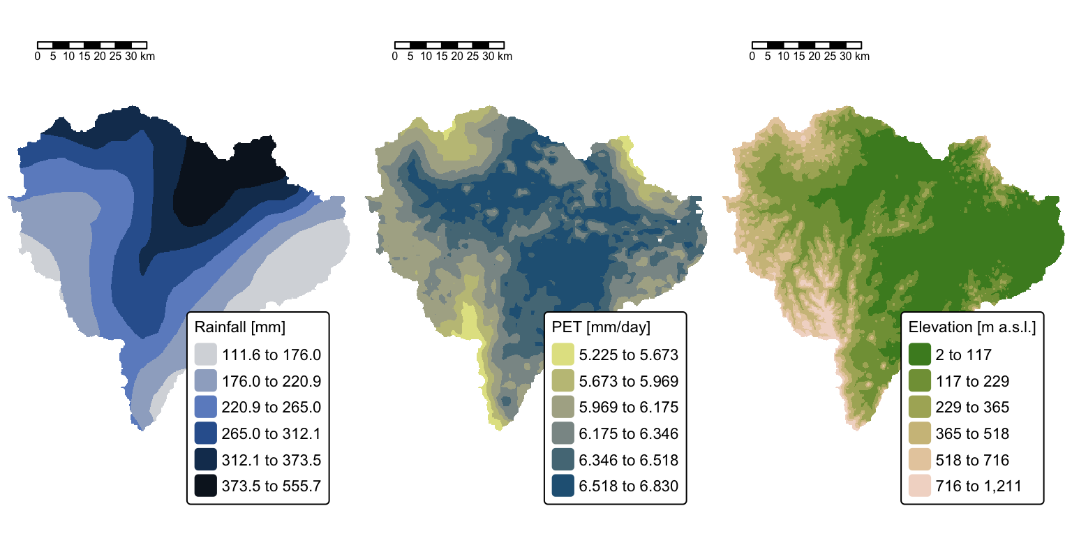
Calculate mass flux
The next block of R code calculates surface runoff using the
D8MassFlux tool from the WhiteboxTools library
accessed in R using the wbt_d8_mass_flux() function.
This tool calculates mass flux using DEM-based surface flow-routing (D8 flow direction from a depressionless DEM). It can model the distribution of materials like sediment or water in a catchment. Users must provide rasters for loading, efficiency, absorption, and an output raster. Unlike standard flow accumulation, this method routes mass, based on the loading raster. Losses are defined by the efficiency raster (proportional, 0–1 or %) and the absorption raster (absolute quantity, same units as loading). The mass transferred between cells is calculated using the following equation:
\[\text{Mass}_{[\textbf{Out}]} = \left(\text{Loading} - \text{Absorption} + \text{Mass}_{[\textbf{In}]}\right) \times \text{Efficiency}\]
In the case of surface runoff:
- \(\text{Loading}\) = rainfall
- \(\text{Absorption}\) = PET + infiltration (in our case only PET)
# Paths to input layers
dem_bris <- "./data/dump/flood/qld_dem_brisbane.tif"
rain_bris <- "./data/dump/flood/qld_rain250m.tif"
pet_bris <- "./data/dump/flood/qld_pet250m.tif"

# Output raster
runoff <- "./data/dump/flood/qld_runoff_mm.tif"
runoff_pet <- "./data/dump/flood/qld_runoff_pet_mm.tif"

# Create dummy rasters for efficiency and absorption
eff_rast <- rast(brisbane_dem)
values(eff_rast) <- 1          # Set values to 1
eff_rast <- mask(eff_rast, brisbane_mask)

abs_rast <- rast(brisbane_dem)
values(abs_rast) <- 0          # Set values to 0
abs_rast <- mask(abs_rast, brisbane_mask)

# Write dummy rasters to disk
writeRaster(eff_rast, "./data/dump/flood/qld_eff_dummy.tif", overwrite = TRUE)
writeRaster(abs_rast, "./data/dump/flood/qld_abs_dummy.tif", overwrite = TRUE)

#Paths to dummy rasters
eff_rast <- "./data/dump/flood/qld_eff_dummy.tif"
abs_rast <- "./data/dump/flood/qld_abs_dummy.tif"

# Calculate runoff in mm with no evapotranspiration
wbt_d8_mass_flux(
    dem = dem_bris,
    loading = rain_bris,
    efficiency = eff_rast,
    absorption = abs_rast,
    output = runoff
)

# Calculate runoff in mm with evapotranspiration
wbt_d8_mass_flux(
    dem = dem_bris,
    loading = rain_bris,
    efficiency = eff_rast,
    absorption = pet_bris,
    output = runoff_pet
)
Plot results on a map:
#Create a SpatRaster stack
r1 <- rast("./data/dump/flood/qld_runoff_mm.tif")
r2 <- rast("./data/dump/flood/qld_runoff_pet_mm.tif")
runoff_stack <- c(r1, r2)

#Convert from mm to gigalitres (GL)
runoff_gl <- (runoff_stack * 62500) / 1e9 # 62500 is area of 250 m pixel

# Define elements and their full names
layer_names <- c("qld_runoff_mm", "qld_runoff_pet_mm")

facet_names <- c(qld_runoff_mm = "Runoff without PET",
                qld_runoff_pet_mm = "Runoff with PET"
               )

# Set the names for each layer to be used as facet labels.
names(runoff_gl) <- paste0(facet_names[layer_names])

# Set tmap to static mode
tmap_mode("plot")

# Create faceted map of runoff
tm_shape(runoff_gl) +
  tm_raster(col.scale = tm_scale_continuous_log(values = "-scico.oslo", n = 4),
            col.legend = tm_legend(title = "Surface Runoff \n[gigalitres]",
                                   position = tm_pos_out("right", "center")),
            col.free = FALSE) +  # Add one common legend
tm_layout(frame = FALSE,
          legend.text.size = 0.7,
          legend.title.size = 0.7,
          legend.position = c("right", "bottom"),
          legend.bg.color = "white",
          panel.label.bg.color = 'linen') +
tm_scalebar(position = c("right", "bottom"), width = 10) + # Add scalebar
tm_facets(ncol = 2, free.scales = FALSE) # Plot each raster as a facet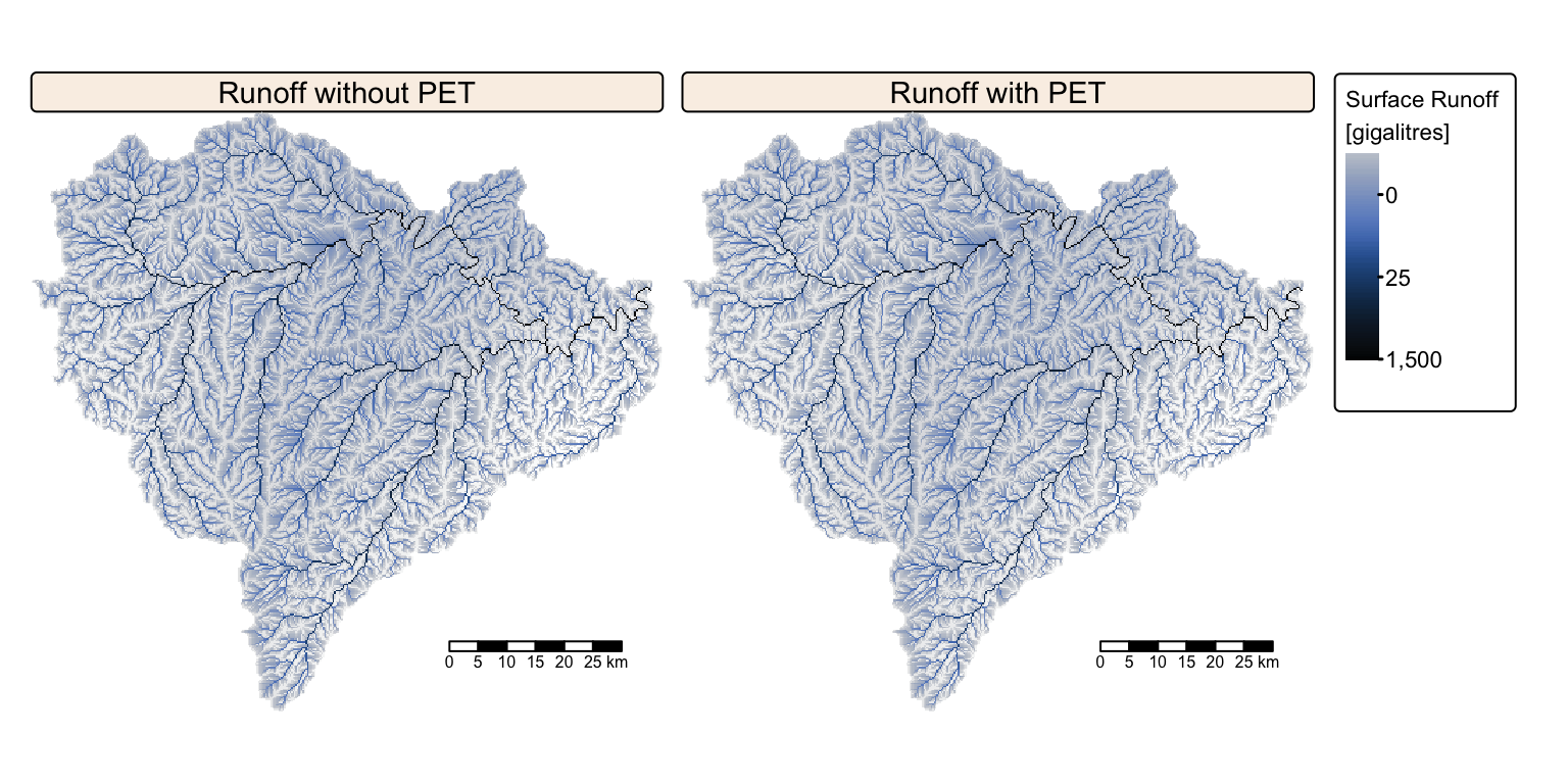
Interrogate runoff rasters
The two surface runoff rasters look identical. The following block of R code reads and prints the maximum runoff values (i.e., the surface runoff recorded at the basin outlet).
# Get the max value
max_val <- global(runoff_gl, fun = "max", na.rm = TRUE)

# Print the max value
head(max_val)
The subsequent block of code extracts estimated total surface runoff values for a list of population centres along the Lockyer, Bremer, and Brisbane rivers, that were affected by flooding during the 10-11 January extreme rainfall event.
# Extract towns of interest
pop_list <- c("Helidon", "Grantham", "Gatton", "Ipswich", "Brisbane")
pop_flood <- brisbane_cities_proj %>%
  filter(name %in% pop_list) %>%
  select(c("name", attr(brisbane_cities_proj, "sf_column")))

# Write list of towns to disk
st_write(pop_flood, "./data/dump/flood/qld_pop_flood_raw.shp", delete_dsn = TRUE)
## Deleting source `./data/dump/flood/qld_pop_flood_raw.shp' using driver `ESRI Shapefile'
## Writing layer `qld_pop_flood_raw' to data source
## `./data/dump/flood/qld_pop_flood_raw.shp' using driver `ESRI Shapefile'
## Writing 5 features with 1 fields and geometry type Point.# Filter stream network raster to only include values with Strahler n > 3
stream_network <- rast(qld_streams)
strahler_ifel <- ifel(strahler < 4, NA, stream_network)
writeRaster(strahler_ifel, "./data//dump/flood/qld_stream_s4.tif", overwrite = TRUE)
# Path to files
flood_pop_raw <- "./data/dump/flood/qld_pop_flood_raw.shp"
flood_pop_snapped <- "./data/dump/flood/qld_pop_flood_snap.shp"
brisbane_streams <- "./data/dump/flood/qld_stream_s4.tif"
# Snap towns to stream network
wbt_jenson_snap_pour_points(
pour_pts = flood_pop_raw,
streams = brisbane_streams,
output = flood_pop_snapped,
snap_dist = 20000 # Maximum snap distance in map units
)
# Load snapped towns
pop_flood_snapped <- st_read(flood_pop_snapped)## Reading layer `qld_pop_flood_snap' from data source
## `/Volumes/Work/Dropbox/Transfer/SCII206/R-Resource/data/dump/flood/qld_pop_flood_snap.shp'
## using driver `ESRI Shapefile'
## Simple feature collection with 5 features and 1 field
## Geometry type: POINT
## Dimension: XY
## Bounding box: xmin: 1954957 ymin: -3159522 xmax: 2042957 ymax: -3143022
## Projected CRS: GDA94 / Australian Albers# Extract surface runoff values
# Ensure both objects share the same CRS
if (st_crs(pop_flood_snapped)$proj4string != crs(runoff_gl)) {
pop_flood_snapped <- st_transform(pop_flood_snapped, crs(runoff_gl))
}
# Add an ID column to preserve the row order during merging
pop_flood_snapped <- pop_flood_snapped %>% mutate(ID = row_number())
# Extract raster values; the first column 'ID' corresponds to the point IDs,
# and the remaining columns are named after the raster layers.
extracted_vals <- terra::extract(runoff_gl, pop_flood_snapped)
# Merge the extracted raster values with the original sf object based on the ID.
pop_flood_snapped <- left_join(pop_flood_snapped, extracted_vals, by = "ID")
# Remove the auxiliary ID column if no longer needed
pop_flood_snapped$ID <- NULL
# Print runoff values
head(pop_flood_snapped)Summary
In this practical exercise, we estimated the total surface runoff generated within the Brisbane River catchment in response to the extreme rainfall event of 10–11 January 2011. Daily rainfall data from the Bureau of Meteorology (BoM) and a 250 m resolution digital elevation model (DEM) from Geoscience Australia were used to route flow and compute runoff, employing the hydrological modelling tools provided by the WhiteboxTools library accessed in R via the whitebox package. For the initial calculations, we assumed that both evaporation and infiltration were negligible during the event, thereby converting all rainfall directly into surface runoff. Subsequently, a global dataset of potential evapotranspiration was incorporated to estimate the evaporation that may have occurred, leading to revised runoff calculations.
List of R functions
This practical showcased a diverse range of R functions. A summary of these is presented below:
base R functions
apply(): applies a function to the margins (rows, columns, etc.) of an array or matrix. It is frequently used for performing vectorised operations across the dimensions of structured data.c(): concatenates its arguments to create a vector, which is one of the most fundamental data structures in R. It is used to combine numbers, strings, and other objects into a single vector.cbind(): binds objects by columns to form a matrix or data frame. It ensures that the input objects have matching row dimensions and aligns them side by side.head(): returns the first few elements or rows of an object, such as a vector, matrix, or data frame. It is a convenient tool for quickly inspecting the structure and content of data.length(): returns the number of elements in a vector or list. It is a basic utility for checking the size or dimensionality of an object.paste0(): concatenates strings without any separator, forming a single character string. It is useful for dynamically generating labels, file names, or messages.seq_along(): generates a sequence of integers from 1 to the length of its argument. It is widely used to create indices when iterating over elements of a vector or list.sum(): adds together all the elements in its numeric argument. It is one of the most straightforward arithmetic functions used to compute totals.is.na(): tests each element of its argument for the presence of a missing value (NA). It is a crucial function for data cleaning and for handling incomplete datasets.
dplyr (tidyverse) functions
%>%(pipe operator): passes the output of one function directly as the input to the next, creating a clear and readable chain of operations. It is a hallmark of the tidyverse, promoting an intuitive coding style.filter(): subsets rows of a data frame based on specified logical conditions. It is essential for extracting relevant data for analysis.left_join(): merges two data frames by including all rows from the left data frame and matching rows from the right. It is commonly used to retain all observations from the primary dataset while incorporating additional information.mutate(): adds new columns or transforms existing ones within a data frame. It is essential for creating derived variables and modifying data within the tidyverse workflow.row_number(): generates a sequential ranking of rows, often used to create unique identifiers. It is particularly useful within grouped operations to order or index rows.select(): extracts a subset of columns from a data frame based on specified criteria. It simplifies data frames by keeping only the variables needed for analysis.
grid functions
unit(): constructs unit objects that specify measurements for graphical parameters, such as centimeters or inches. It is often used in layout and annotation functions for precise control over plot elements.
sf functions
st_coordinates(): extracts the coordinate matrix from an sf object, providing a numeric representation of spatial locations. It is often used when the coordinates need to be manipulated separately from the geometry.st_buffer(): creates a buffer zone around spatial features by a specified distance. It is useful for spatial analyses that require proximity searches or zone creation.st_intersects(): checks if geometries in one sf object intersect with geometries in another, returning a logical or sparse matrix of the results. This function underpins many spatial analyses by identifying overlapping or touching features.st_point(): generates point geometries from a vector of coordinates, representing specific locations in space. It is widely used for mapping individual locations or creating simple spatial objects.st_read(): reads spatial data from a file (such as shapefiles, GeoJSON, or GeoPackages) into an sf object. It is the primary method for importing external geospatial data into R.st_sfc(): creates a simple feature geometry list column from one or more geometries. It is used to construct sf objects from raw geometrical inputs.st_sf(): converts a regular data frame into an sf object by attaching spatial geometry information. It is the foundational step for performing spatial analysis using the simple features framework.st_transform(): reprojects spatial data into a different coordinate reference system. It ensures consistent spatial alignment across multiple datasets.st_union(): merges multiple spatial geometries into a single combined geometry. It is useful for dissolving boundaries and creating aggregate spatial features.st_write(): writes an sf object to an external file in various formats, such as shapefiles or GeoPackages. It is used to export spatial data for sharing or use in other applications.
terra functions
as.polygons(): converts a raster object into polygon features, effectively vectorising the raster cells. It is useful when analyses require the conversion of continuous raster data into discrete polygon objects.crs(): retrieves or sets the coordinate reference system for spatial objects such as SpatRaster or SpatVector. It is essential for proper projection and alignment of spatial data.crop(): trims a raster to a specified spatial extent. It is used to focus analysis on a region of interest within a larger dataset.extract(): retrieves cell values from a SpatRaster at specified locations given by a SpatVector. It is widely used for sampling raster data based on point or polygon geometries.global(): computes summary statistics, such as mean or sum, for the cells in a SpatRaster across its entire extent. It provides a quick overview of the raster data’s overall characteristics.ifel(): performs element-wise conditional operations on raster data, similar to an if-else statement. It creates new rasters based on specified conditions.mask(): applies a mask to a raster using a vector or another raster, setting cells outside the desired area to NA. It is useful for isolating specific regions within a dataset.names(): gets or sets the names of layers within a SpatRaster object. It facilitates easier reference and manipulation of individual raster layers.project(): reprojects spatial data from one CRS to another, enabling alignment of datasets. It is essential for working with spatial data from different sources.rast(): creates a new SpatRaster object or converts data into a raster format. It is the entry point for handling multi-layered spatial data in terra.resample(): changes the resolution or alignment of a SpatRaster by resampling its values to match a template raster. It ensures that multiple raster datasets are spatially consistent for analysis.values(): retrieves or assigns the cell values of a SpatRaster. It allows direct manipulation of the underlying data in the raster.vect(): converts various data types into a SpatVector object for vector spatial analysis. It supports points, lines, and polygons for versatile spatial data manipulation.writeRaster(): writes a raster object to disk in various file formats, including GeoTIFF. It allows users to export processed raster data for sharing, further analysis, or use in other software environments.
tmap functions
tm_borders(): draws border lines around spatial objects on a map. It is often used in combination with fill functions to delineate regions clearly.tm_facets(): arranges multiple maps into facets based on a grouping variable, enabling side‑by‑side comparisons. It is particularly useful for exploring differences across categories within a dataset.tm_fill(): fills spatial objects with color based on data values or specified aesthetics in a tmap. It is a key function for thematic mapping.tm_labels(): adds text labels to map features based on specified attributes in tmap. It is useful for annotating spatial data to improve map readability.tm_layout(): customises the overall layout of a tmap, including margins, frames, and backgrounds. It provides fine control over the visual presentation of the map.tm_legend(): customises the appearance and title of map legends in tmap. It is used to enhance the clarity and presentation of map information.tm_pos_out(): positions map elements such as legends or scale bars outside the main map panel. It helps reduce clutter within the map area.tm_raster(): adds a raster layer to a map with options for transparency and color palettes. It is tailored for visualizing continuous spatial data.tm_scale_categorical(): applies a categorical color scale to represent discrete data in tmap. It is ideal for mapping data that fall into distinct classes.tm_scale_continuous(): applies a continuous color scale to a raster layer in tmap. It is suitable for representing numeric data with smooth gradients.tm_scale_continuous_log(): applies a logarithmically transformed continuous colour scale to raster data in a tmap. It is beneficial for data that cover several orders of magnitude, enhancing visual distinction.tm_scale_intervals(): creates a custom interval-based color scale for a raster layer in tmap. It enhances visualization by breaking data into meaningful ranges.tm_scalebar(): adds a scale bar to a tmap to indicate distance. It can be customised in terms of breaks, text size, and position.tm_shape(): defines the spatial object that subsequent tmap layers will reference. It establishes the base layer for building thematic maps.tm_symbols(): adds point symbols to a map with customizable shapes, sizes, and colors based on data attributes. It is useful for plotting locations with varying characteristics.tmap_arrange(): arranges multiple tmap objects into a single composite layout. It is useful for side-by-side comparisons or dashboard displays.tmap_mode(): switches between static (“plot”) and interactive (“view”) mapping modes in tmap. It allows users to choose the most appropriate display format for their needs.
whitebox functions
wbt_init(): initialises the WhiteboxTools environment within R by setting up the necessary configurations and paths. It must be run before any Whitebox geoprocessing functions are used.wbt_breach_depressions_least_cost(): removes depressions (or sinks) in a DEM by identifying least-cost breach paths, thereby conditioning the DEM for hydrological modelling. It modifies the elevation data so that water can flow more naturally across the surface.wbt_d8_flow_accumulation(): computes the flow accumulation from a D8 flow pointer raster using WhiteboxTools. It calculates how many cells contribute flow to each cell, a key step in watershed analysis.wbt_d8_mass_flux(): computes the mass flux based on a DEM, loading, efficiency, and absorption using the D8 algorithm. It is used to estimate surface runoff or related hydrological variables within a terrain.wbt_d8_pointer(): generates a D8 flow direction pointer raster from a DEM using WhiteboxTools. It assigns directional codes to each cell based on the steepest descent path, facilitating subsequent hydrological analyses.wbt_extract_streams(): identifies stream channels by thresholding flow accumulation on a D8 flow accumulation raster. It isolates the stream network, facilitating the extraction of drainage patterns from the terrain.wbt_fill_depressions(): fills depressions in a DEM to eliminate sinks and ensure hydrological connectivity using WhiteboxTools. It raises the elevation of low-lying cells to a level that permits continuous flow.wbt_jenson_snap_pour_points(): adjusts the location of pour points by snapping them to the nearest stream cell based on a specified maximum snap distance. It increases the accuracy of watershed delineation by aligning pour points with the drainage network.wbt_strahler_stream_order(): assigns Strahler stream orders to a drainage network using WhiteboxTools, ranking streams by hierarchy. It is a standard method for classifying stream size and network complexity in hydrological studies.wbt_watershed(): delineates watershed basins from a flow direction raster using WhiteboxTools. It identifies the catchment areas that drain to specified pour points, essential for hydrological analysis and water resource management.