Case Study: The impact of climate change on the distribution of rainfed crops in NSW
SCII205: Introductory Geospatial Analysis / Practical No. 6
Alexandru T. Codilean
Last modified: 2025-06-14
![]()
Introduction
In this practical we are using gridded weather data from the Bureau of Meteorology (BOM) and land cover data from Geoscience Australia (GA) to explore how precipitation and temperature patterns have changed over the past 30 years in Australia, and how these changes might have affected rainfed crops in NSW.
R packages
The practical will primarily utilise R functions from packages explored in previous sessions:
The tidyverse: is a collection of R packages designed for data science, providing a cohesive set of tools for data manipulation, visualization, and analysis. It includes core packages such as ggplot2 for visualization, dplyr for data manipulation, tidyr for data tidying, and readr for data import, all following a consistent and intuitive syntax.
The sf package: provides a standardised framework for handling spatial vector data in R based on the simple features standard (OGC). It enables users to easily work with points, lines, and polygons by integrating robust geospatial libraries such as GDAL, GEOS, and PROJ.
The terra package: is designed for efficient spatial data analysis, with a particular emphasis on raster data processing and vector data support. As a modern successor to the raster package, it utilises improved performance through C++ implementations to manage large datasets and offers a suite of functions for data import, manipulation, and analysis.
The tmap package: provides a flexible and powerful system for creating thematic maps in R, drawing on a layered grammar of graphics approach similar to that of ggplot2. It supports both static and interactive map visualizations, making it easy to tailor maps to various presentation and analysis needs.
Resources
- The Geocomputation with R book.
- The tidyverse library of packages documentation.
- The sf package documentation.
- The terra package documentation.
- The tmap package documentation.
Obtaining data
All data to be used in this practical has already been downloaded and is provided to you as part of the data package that comes with this information document. For completeness, however, the following sections provide information on how to download data from BOM and GA.
Downloading data from BOM
The gridded precipitation and temperature data used in this practical is freely available from the BOM website:
- Decadal and multi-decadal rainfall
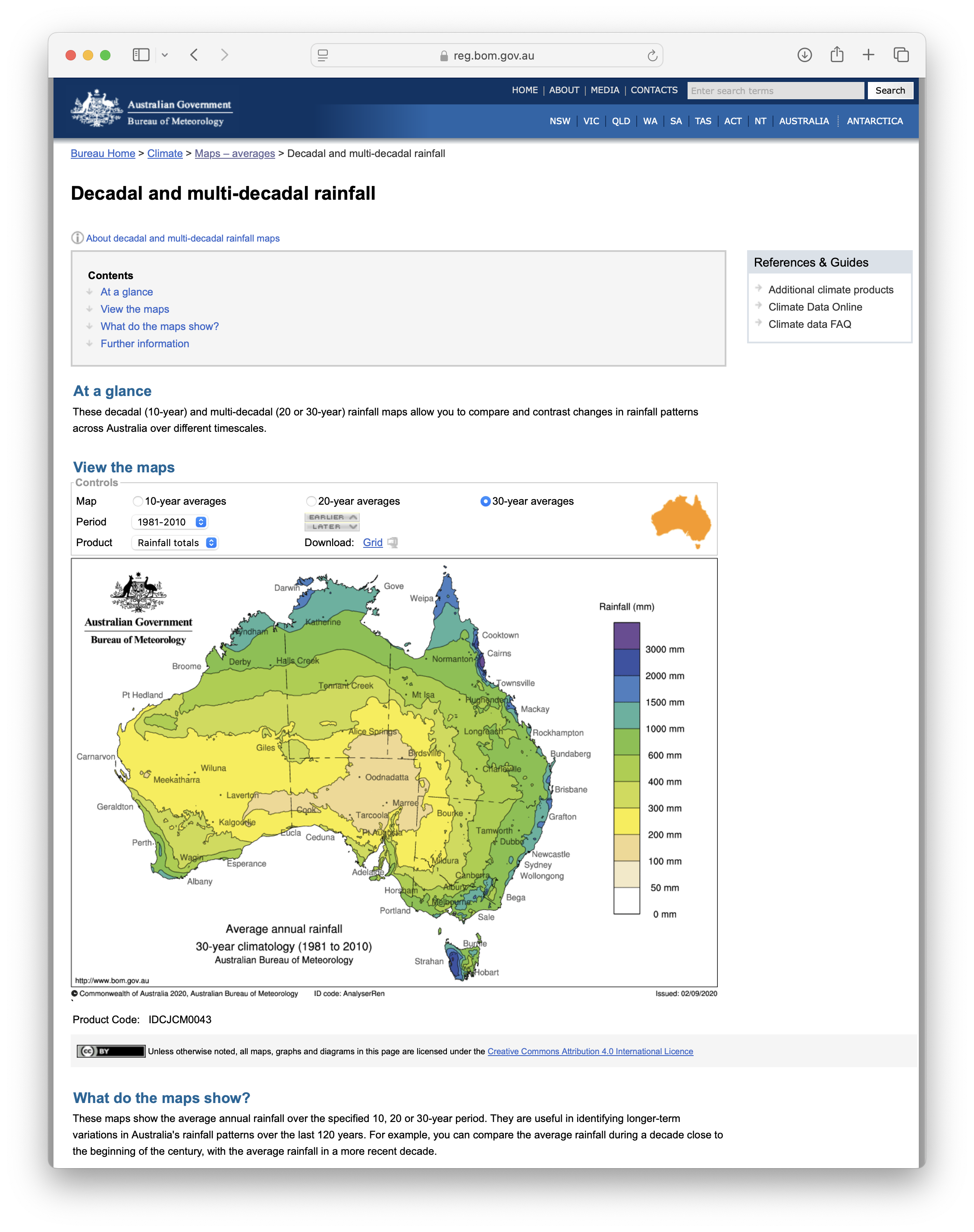
- Decadal and multi-decadal temperature
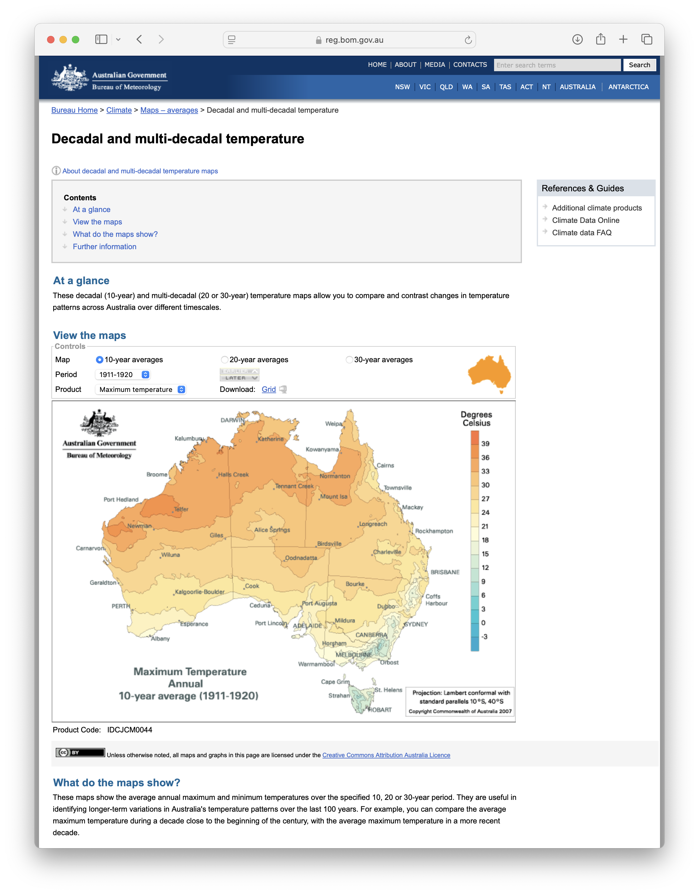
To download data, select the desired period and product, and then
click on Download: Grid
Downloading data from GA
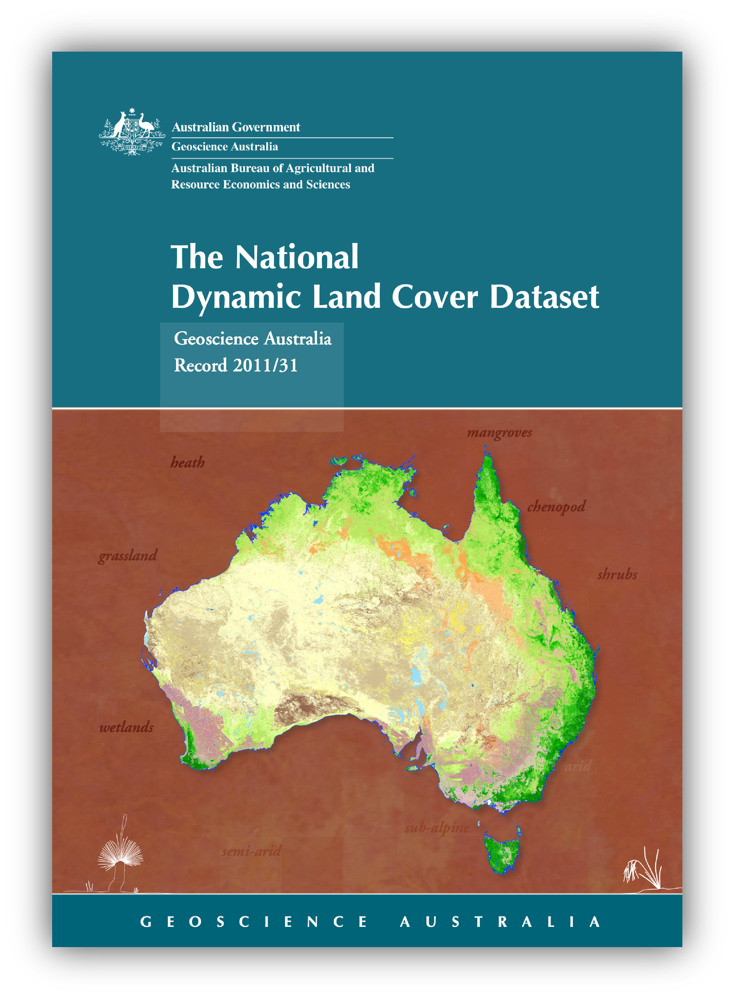
Geoscience Australia provides access to a wide range of geospatial data. In this practical, we are interested in the The National Dynamic Land Cover Dataset that thematically illustrates Australian land cover divided into 34 different land cover classes. These range from cultivated and managed land covers (crops and pastures) to natural land covers such as forest and grasslands. It also provides raster layers showing trends in the annual minimum, mean, and maximum Enhanced Vegetation Index (EVI) from 2000 to 2008. The EVI is an index created from satellite data and is useful in determining vegetation health and density.
The dataset is available from this page.

Load necessary R packages
All necessary packages should be installed already, but just in case:
# Main spatial packages
install.packages("sf")
install.packages("terra")

# tmap dev version
install.packages("tmap", repos = c("https://r-tmap.r-universe.dev",
                                   "https://cloud.r-project.org"))
# leaflet for dynamic maps
install.packages("leaflet"

# tidyverse for additional data wrangling
install.packages("tidyverse")
Load packages:
Trends in rainfall
We are provided with two precipitation datasets:
- Gridded average decadal rainfall for the period 1971 to 1980
- Gridded average decadal rainfall for the period 1996 to 2005
To investigate how the spatial distribution and amount of precipitation have changed over time, we will subtract the 1971-1980 dataset from the 1996-2005 dataset.
Read in rainfall data
The gridded rainfall data is provided by the BOM in ESRI ASCII raster format. More information about this format can be found here.
We can use the rast() function in terra
to read in the two precipitation grids:
# Specify the path to your ESRI ASCII file
rain_71to80 <- "./data/data_crops/raster/BOM/Rainfall/r7180.txt"
rain_96to05 <- "./data/data_crops/raster/BOM/Rainfall/r9605.txt"

# Read in the ESRI ASCII files
rast_rain_71to80 <- rast(rain_71to80)
rast_rain_96to05 <- rast(rain_96to05)

# Change the name of the layer to "Rainfall"
names(rast_rain_71to80) <- "Rainfall"
names(rast_rain_96to05) <- "Rainfall"

# Print a summary of the two rasters to verify metadata
print(rast_rain_71to80)
## class : SpatRaster
## dimensions : 691, 886, 1 (nrow, ncol, nlyr)
## resolution : 0.05, 0.05 (x, y)
## extent : 111.975, 156.275, -44.525, -9.975 (xmin, xmax, ymin, ymax)
## coord. ref. : lon/lat WGS 84 (CRS84) (OGC:CRS84)
## source : r7180.txt
## name : Rainfall## class : SpatRaster
## dimensions : 691, 886, 1 (nrow, ncol, nlyr)
## resolution : 0.05, 0.05 (x, y)
## extent : 111.975, 156.275, -44.525, -9.975 (xmin, xmax, ymin, ymax)
## coord. ref. : lon/lat WGS 84 (CRS84) (OGC:CRS84)
## source : r9605.txt
## name : Rainfall# Plot rasters for quick visual inspection
rain_map1 <-
tm_shape(rast_rain_71to80) +
tm_raster("Rainfall",
col.scale = tm_scale_continuous(values = "pu_gn_div"),
col.legend = tm_legend(title = "Rainfall [mm]",
position = tm_pos_out(cell.h = "center", cell.v = "bottom"),
orientation = "landscape")
) +
tm_layout(frame = FALSE)
rain_map2 <-
tm_shape(rast_rain_96to05) +
tm_raster("Rainfall",
col.scale = tm_scale_continuous(values = "pu_gn_div"),
col.legend = tm_legend(title = "Rainfall [mm]",
position = tm_pos_out(cell.h = "center", cell.v = "bottom"),
orientation = "landscape")
) +
tm_layout(frame = FALSE)
# Two maps side by side
tmap_arrange(rain_map1, rain_map2)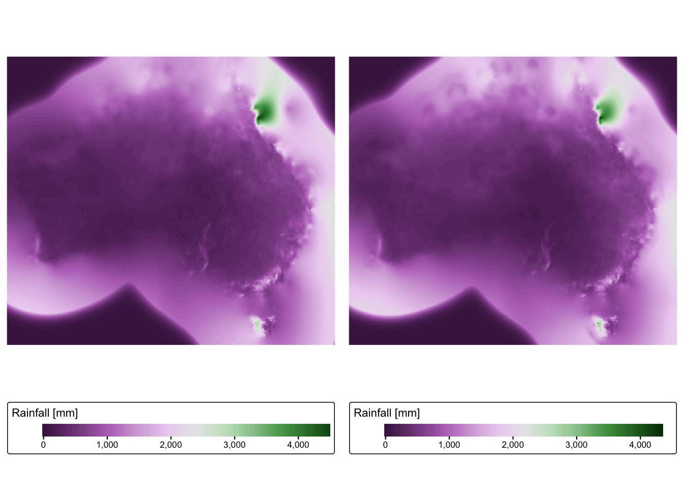
A quick inspection of the output reveals the following:
Coordinate system: R has correctly guessed that the data are in geographic coordinates (i.e., lat/long), however it has incorrectly assigned these coordinates to the WGS 84 datum. BOM data are in fact referenced to the Geocentric Datum of Australia 1994 (GDA1994) datum.
Resolution: The data has a grid spacing of 0.05. Given that the data is in geographic coordinates, the units are in arc degrees, and so the spatial resolution of the rainfall data is 0.05 arc decimal degrees. This corresponds to roughly 5 km at the equator.
Extent: It is obvious from the two plots that the data extends beyond the coastline of Australia. Given that the grids are obtained by interpolation of weather station data, it is likely that interpolated values extending beyond the coastline are unreliable.
In the following steps, we will rectify the coordinate system and extent issues and project the data into a metric coordinate system so that calculations performed on the data will be planimetrically correct.
Assign and change projection
# Define the CRS as Geocentric Datum of Australia 1994 (GDA94) using the EPSG code 4283
crs(rast_rain_71to80) <- "EPSG:4283"
crs(rast_rain_96to05) <- "EPSG:4283"

# Print a summary of the two rasters to verify correct datum assignment
print(rast_rain_71to80)
## class : SpatRaster
## dimensions : 691, 886, 1 (nrow, ncol, nlyr)
## resolution : 0.05, 0.05 (x, y)
## extent : 111.975, 156.275, -44.525, -9.975 (xmin, xmax, ymin, ymax)
## coord. ref. : lon/lat GDA94 (EPSG:4283)
## source : r7180.txt
## name : Rainfall## class : SpatRaster
## dimensions : 691, 886, 1 (nrow, ncol, nlyr)
## resolution : 0.05, 0.05 (x, y)
## extent : 111.975, 156.275, -44.525, -9.975 (xmin, xmax, ymin, ymax)
## coord. ref. : lon/lat GDA94 (EPSG:4283)
## source : r9605.txt
## name : RainfallTo reproject spatial data, R interfaces with the PROJ open source C++ library that transforms coordinates from one coordinate reference system (CRS) to another.
There are two ways to define or identify a given CRS:
Using the PROJ ‘proj-string’ that contains information identifying the CRS and its main parameters. Examples include:
+proj=aea +lat_1=0 +lat_2=-30 +lon_0=130and+proj=robin, as used in Practical No. 2.Using an identifying ‘authority:code’ text string, such as
EPSG:4283. Lists of EPSG codes are provided here: https://epsg.io and here https://spatialreference.org
Both of the above methods should work, but sticking to the EPSG code might be desirable as it is widely recognised and used, and it is also future-proof. For more information about this topic see Chapter 7 of the Geocomputation with R book.
The following chunk of code will reproject the two rasters to Australian Albers equal area projection referenced to the GDA94 datum. The EPSG code for this projection is 3577
rain_71to80_proj <- project(rast_rain_71to80,
        "EPSG:3577",             # Australian Albers / GDA94
        method = "bilinear",     # bilinear interpolation for continuous data
        res = 5000,              # 5000 m = 5 km resolution
        mask=TRUE)

rain_96to05_proj <- project(rast_rain_96to05,
        "EPSG:3577",
        method = "bilinear",
        res = 5000,
        mask=TRUE)

# Print a summary of the two rasters to verify new CRS
print(rain_71to80_proj)
## class : SpatRaster
## dimensions : 801, 994, 1 (nrow, ncol, nlyr)
## resolution : 5000, 5000 (x, y)
## extent : -2248922, 2721078, -5052873, -1047873 (xmin, xmax, ymin, ymax)
## coord. ref. : GDA94 / Australian Albers (EPSG:3577)
## source(s) : memory
## name : Rainfall
## min value : 0.000
## max value : 4756.792## class : SpatRaster
## dimensions : 801, 994, 1 (nrow, ncol, nlyr)
## resolution : 5000, 5000 (x, y)
## extent : -2248922, 2721078, -5052873, -1047873 (xmin, xmax, ymin, ymax)
## coord. ref. : GDA94 / Australian Albers (EPSG:3577)
## source(s) : memory
## name : Rainfall
## min value : 0.000
## max value : 4346.445# Plot rasters for quick visual inspection
rain_map1 <-
tm_shape(rain_71to80_proj) +
tm_raster("Rainfall",
col.scale = tm_scale_continuous(values = "pu_gn_div"),
col.legend = tm_legend(title = "Rainfall [mm]",
position = tm_pos_out(cell.h = "center", cell.v = "bottom"),
orientation = "landscape")
) +
tm_layout(frame = FALSE)
rain_map2 <-
tm_shape(rain_96to05_proj) +
tm_raster("Rainfall",
col.scale = tm_scale_continuous(values = "pu_gn_div"),
col.legend = tm_legend(title = "Rainfall [mm]",
position = tm_pos_out(cell.h = "center", cell.v = "bottom"),
orientation = "landscape")
) +
tm_layout(frame = FALSE)
# Two maps side by side
tmap_arrange(rain_map1, rain_map2)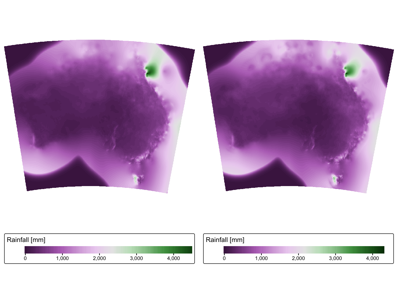
Crop rasters to coastline
To crop a raster to an extent defined by another dataset (in our case
a vector dataset representing the coastline of Australia), we can use
the crop() and mask() functions in
terra.
First we need to load the coastline data and inspect:
# Read in shapefile
aus_coast <- read_sf("./data/data_crops/vector/shapefile/bnd_GDA94.shp")

# Print a summary of the shapefile
print(aus_coast)
## Simple feature collection with 9 features and 13 fields
## Geometry type: POLYGON
## Dimension: XY
## Bounding box: xmin: 113.1563 ymin: -43.64305 xmax: 153.6386 ymax: -10.68758
## Geodetic CRS: GDA94
## # A tibble: 9 × 14
## OBJECTID FEATTYPE STATE FEATREL ATTRREL PLANACC SOURCE CREATED
## <dbl> <chr> <chr> <date> <date> <int> <chr> <date>
## 1 1 Mainland TAS 2003-03-11 2003-03-11 9999 GEOSCIENCE A… 2006-05-09
## 2 2 Mainland NT 2002-06-29 2002-06-29 9999 GEOSCIENCE A… 2006-05-09
## 3 3 Mainland WA 2004-08-09 2004-08-09 9999 GEOSCIENCE A… 2006-05-09
## 4 4 Mainland SA 2003-08-01 2003-08-01 9999 GEOSCIENCE A… 2006-05-09
## 5 5 Mainland VIC 2000-12-12 2000-12-12 9999 GEOSCIENCE A… 2006-05-09
## 6 6 Mainland QLD 2002-10-31 2002-10-31 9999 GEOSCIENCE A… 2006-05-09
## 7 7 Mainland JBT 2003-07-05 2003-07-05 9999 GEOSCIENCE A… 2006-05-09
## 8 8 Mainland ACT 2002-08-19 2002-08-19 9999 GEOSCIENCE A… 2006-05-09
## 9 9 Mainland NSW 2004-11-16 2004-11-16 9999 GEOSCIENCE A… 2006-05-09
## # ℹ 6 more variables: RETIRED <date>, PID <dbl>, SYMBOL <int>,
## # SHAPE_Leng <dbl>, SHAPE_Area <dbl>, geometry <POLYGON [°]>From the summary, we can see that aus_coast has several
attribute columns, including one for state and territory names. Plot the
data with the state/territory name column for quick inspection:
# Plot shapefile for quick visual inspection
tm_shape(aus_coast) + tm_fill("STATE") + tm_borders() + tm_layout(frame = FALSE)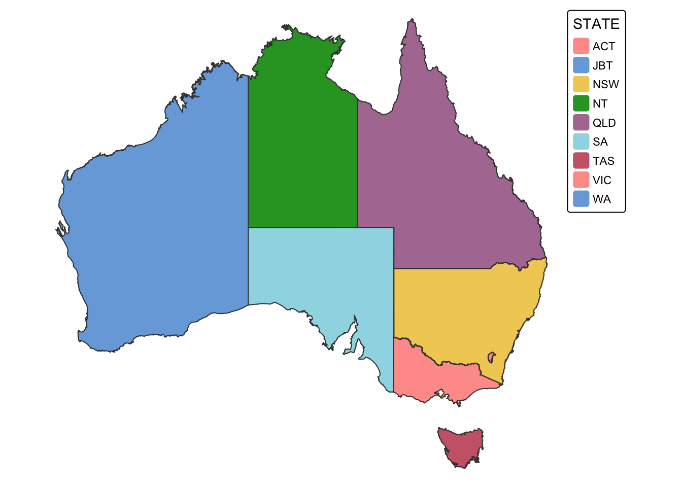
The coastline data needs some processing before we can use it to crop the precipitation rasters:
First, the data needs to be reprojected so that its CRS matches that of the rasters (i.e., EPSG:3577).
Second, we will dissolve all state/territory polygons so that the resulting layer only shows coastlines.
aus_coastalso includes an attribute column (FEATTYPE) that is common for all states and territories and so can be used in the dissolve operation.
Dissolve states and territories with st_union():
# Define the field and value to use for dissolving geometry
coastline = aus_coast[aus_coast$FEATTYPE == "Mainland", ]

# Perform dissolve
aus_coast_diss = st_union(coastline)

# Plot shapefile for quick visual inspection
tm_shape(aus_coast_diss) + tm_fill() + tm_borders() + tm_layout(frame = FALSE)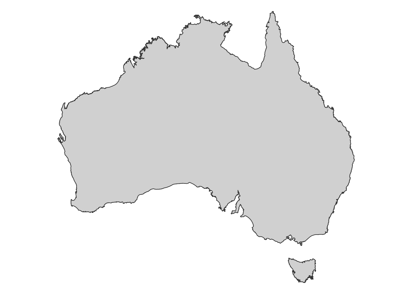
Project dissolved coastline layer to EPSG:3577:
# Transform to EPSG:3577
aus_coast_proj <- st_transform(aus_coast_diss, crs = "EPSG:3577")

# An alternative way of doing the above is:
# aus_coast_proj <- st_transform(aus_coast_diss, st_crs(rain_71to80_proj))
# In this case, the CRS info is read from one of the rainfall rasters

# Plot shapefile for quick visual inspection
tm_shape(aus_coast_proj) + tm_fill() + tm_borders() + tm_layout(frame = FALSE)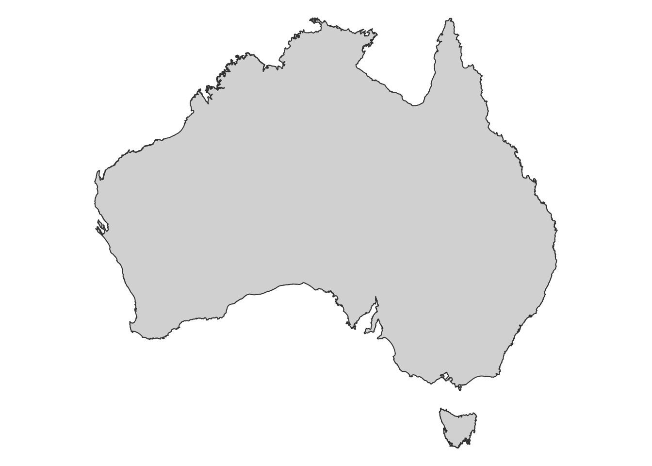
We are now ready to crop the rainfall rasters. For this purpose we
will use two terra functions: crop() and
mask(). The first function reduces the rectangular extent
of the object passed to its first argument based on the extent of the
object passed to its second argument. The second function sets values
outside of the bounds of the object passed to its second argument to
no data.
# Convert sf MULTIPOLYGON geometry object to terra SpatVector object
aus_coast_vect <- vect(aus_coast_proj)

# Crop 71to80 raster
rain_71to80_cropped = crop(rain_71to80_proj, aus_coast_vect)
rain_71to80_final = mask(rain_71to80_cropped, aus_coast_vect)

# Crop 96to05 raster
rain_96to05_cropped = crop(rain_96to05_proj, aus_coast_vect)
rain_96to05_final = mask(rain_96to05_cropped, aus_coast_vect)
Now plot the resulting rasters. Here we will set both maps to show the same colour scale so that map colours are directly comparable:
# Plot rasters using the same limits to colour scale

# Extract raster values for the "Rainfall" layer from both rasters.
# terra::values() returns a matrix, so we extract the column corresponding to "Rainfall".
rain1_vals <- values(rain_71to80_final)[, "Rainfall"]
rain2_vals <- values(rain_96to05_final)[, "Rainfall"]

# Compute the common limits (min and max) across both rasters.
common_limits <- c(
  min(c(rain1_vals, rain2_vals), na.rm = TRUE),
  max(c(rain1_vals, rain2_vals), na.rm = TRUE)
)

# Now create the maps with the same scale limits.
rain_map1 <-
  tm_shape(rain_71to80_final) +
      tm_raster("Rainfall",
          col.scale = tm_scale_continuous_sqrt(values = "pu_gn_div", limits = common_limits),
          col.legend = tm_legend(title = "Rainfall [mm]",
                          position = tm_pos_out(cell.h = "center", cell.v = "bottom"),
                          orientation = "landscape")
                ) +
  tm_layout(frame = FALSE)

rain_map2 <-
  tm_shape(rain_96to05_final) +
      tm_raster("Rainfall",
          col.scale = tm_scale_continuous_sqrt(values = "pu_gn_div", limits = common_limits),
          col.legend = tm_legend(title = "Rainfall [mm]",
                          position = tm_pos_out(cell.h = "center", cell.v = "bottom"),
                          orientation = "landscape")
                ) +
  tm_layout(frame = FALSE)

# Two maps side by side
tmap_arrange(rain_map1, rain_map2)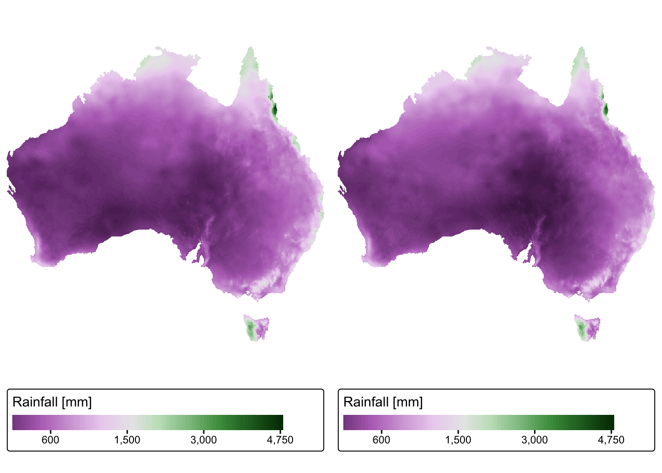
Calculate rainfall difference
Cell-by-cell operations (also known as map or raster algebra) are fully supported by the terra package. To subtract the [1971-1980] raster from the [1996-2005] raster, we simply write:
This operation creates a new SpatRaster object with the
same spatial properties (i.e., resolution, extent, CRS, etc.) as the
input layers.
Next we create a map to show the difference in rainfall values:
# Define bounding box
aus_region =
  st_bbox(c(xmin = 113, xmax = 153,   # X coordinates
            ymin = -45, ymax = -10),  # Y coordinates
          crs = st_crs(4326))         # Define coord. system; 4326: WGS84 lat/long

# Draw map
map_rain <-
  tm_shape(rain_diff, bbox = aus_region) +
      tm_raster("Rainfall",
          col.scale = tm_scale(values = "pu_gn_div"),
          col.legend = tm_legend(title = "Rainfall [mm]",
                          position = tm_pos_out(cell.h = "right", cell.v = "center"),
                          orientation = "portrait")
                )

# Add map elements
map_rain +
  # Use tm_grid() to plot CRS of the object
  # Use tm_graticules() to plot lat/long
  tm_graticules(col = "lightgray", lwd = 0.3) +


  tm_compass(
      type = "arrow",              # Options: "arrow", "4star", "8star", "radar", "rose"
      position = c("left", "top")  # Position of compass:
            ) +                    # "left", "center", "right", for the first value and
                                   # "top", "center", "bottom", for the second value

  tm_scalebar(breaks = c(0, 500, 1000),                      # Scale bar breaks
        text.size = 0.8, position = c("left", "bottom")) +   # Size / position as above

  # See https://r-tmap.github.io for more options
  tm_title("Trends in Rainfall - Australia ",   # Map title
           fontface = "bold")                   # Typeface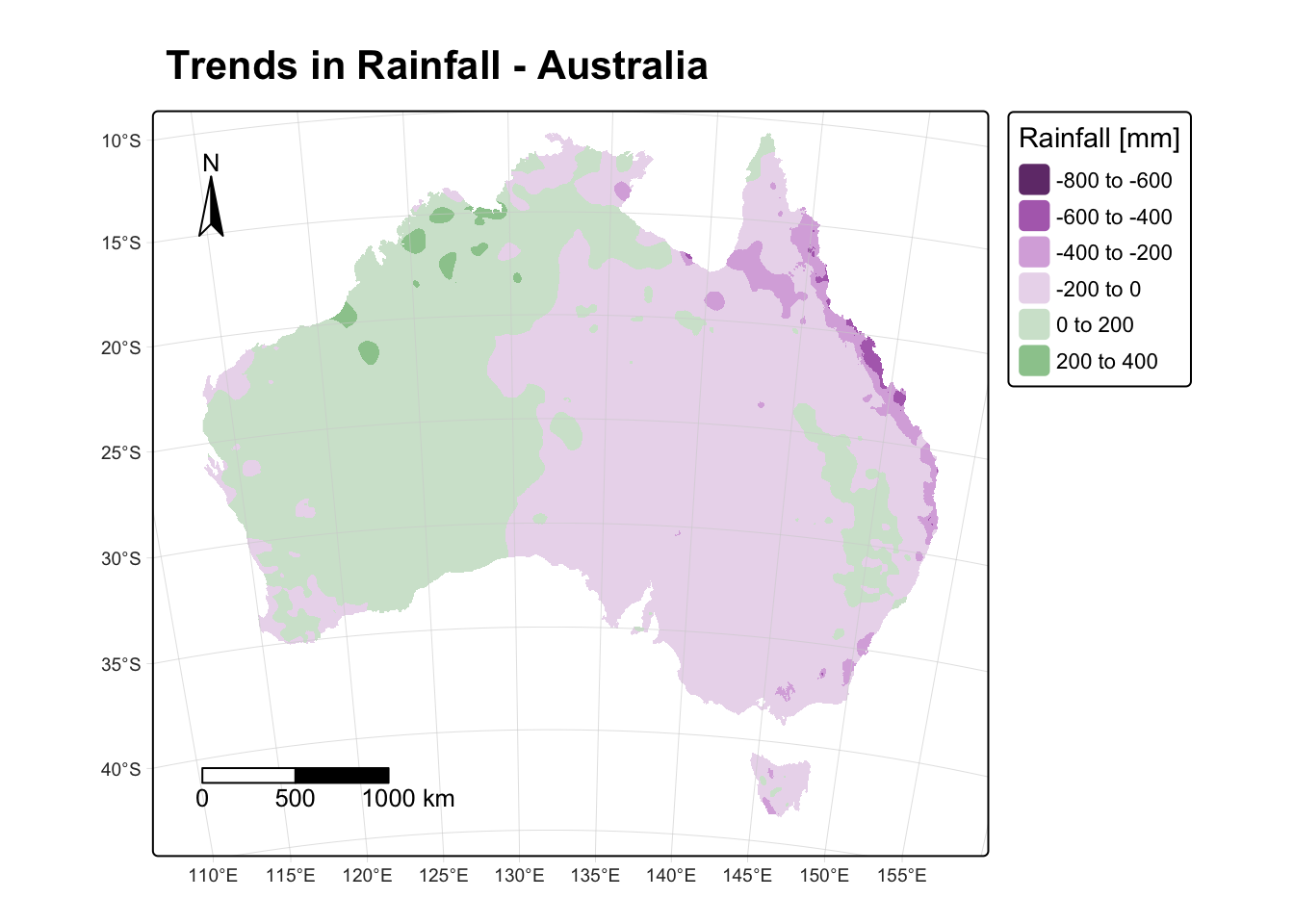
Positive values (shades of green) in the above map show areas where precipitation has increased between the two time periods (e.g., the NW of Australia). Conversely, negative values (shades of purple) show areas where precipitation has decreased between the two periods (e.g., the eastern part of Australia). In summary, the north-western parts of Australia have gotten wetter and the eastern parts drier.
Trends in temperature
For temperature, we are provided with four precipitation datasets:
- Gridded minimum decadal temperature for the periods [1971 to 1980] and [1996 to 2005]
- Gridded maximum decadal temperature for the periods [1971 to 1980] and [1996 to 2005]
To investigate how the spatial distribution and amount of precipitation have changed over time, we will subtract the [1971-1980] min and max datasets from the [1996-2005] min and max dataset.
This is work that you will have to complete in the exercise markdown document provided.
Land cover changes
We will explore changes in land cover using the The National Dynamic Land Cover Dataset (DLCD). This dataset is the first nationally consistent and thematically comprehensive land cover reference for Australia. It is the result of a collaboration between Geoscience Australia and the Australian Bureau of Agriculture and Resource Economics and Sciences, and provides a base-line for identifying and reporting on change and trends in vegetation cover and extent.
The dataset comprises digital files of the land cover classification and three trend datasets showing the change in behaviour of land cover across Australia for the period 2000 to 2008.
As part of this exercise we will use the DLCD
land cover classification data layer to isolate grid cells
that are classed as rainfed crops and then extract mean
greening trends using the enhanced vegetation index (EVI)
data layer for those rainfed crop grid cells.
Read in the DLCD data
The following chunk of code reads in the relevant DLCD data layers:
# Specify the path to your DLCD files
dlcd_classes_file <- "./data/data_crops/raster/DLCD/Scene01-DLCDv1_Class/DLCDv1_Class.tif"
mean_evi_file <- "./data/data_crops/raster/DLCD/Scene01-trend_evi_mean/trend_evi_mean.tif"

# Read in the rasters
dlcd_classes <- rast(dlcd_classes_file)
mean_evi <- rast(mean_evi_file)

#Change the name of the layers to "DLCD_Class" and "EVI"
names(dlcd_classes) <- "DLCD_Class"
names(mean_evi) <- "EVI"

# Print a summary of the two rasters to verify metadata
print(dlcd_classes)
## class : SpatRaster
## dimensions : 14902, 19161, 1 (nrow, ncol, nlyr)
## resolution : 0.002349, 0.002349 (x, y)
## extent : 110, 155.0092, -45.0048, -10 (xmin, xmax, ymin, ymax)
## coord. ref. : lon/lat WGS 84 (EPSG:4326)
## source : DLCDv1_Class.tif
## categories : BinValues, Histogram
## name : DLCD_Class
## min value : 2
## max value : NA## class : SpatRaster
## dimensions : 14902, 19161, 1 (nrow, ncol, nlyr)
## resolution : 0.002349, 0.002349 (x, y)
## extent : 110, 155.0092, -45.0048, -10 (xmin, xmax, ymin, ymax)
## coord. ref. : lon/lat WGS 84 (EPSG:4326)
## source : trend_evi_mean.tif
## name : EVI
## min value : NA
## max value : NAInspecting the information printed above, we can see that both
rasters have the correct CRS information (EPSG:4326), and
so no adjustments are required regarding CRS. However, the
print() function lists both min and max values for
mean_evi as being NA. This occurs when a
raster is too large — in our case trend_evi_mean.tif is
1.15 GB — and so the next chunk of code instructs R to explicitly
calculate the min and max values:
# Compute global statistics (min and max), ignoring NA values.
global_stats <- global(mean_evi, fun = c("min", "max"), na.rm = TRUE)
print(global_stats)
## min max
## EVI -0.09511322 0.08792239To avoid problems with plotting the mean_evi raster, the
next chunk of code forces all grid cells beyond the min and max interval
to NA (i.e., no data):
# Extract all raster values into memory
evivalues <- values(mean_evi)

# Set values > 0.08792239 or < -0.09511322 to NA
evivalues[evivalues > 0.08792239 | evivalues < -0.09511322] <- NA

# Reassign the modified values back to the raster
values(mean_evi) <- evivalues

# Print a summary of the two rasters to verify metadata
print(dlcd_classes)
## class : SpatRaster
## dimensions : 14902, 19161, 1 (nrow, ncol, nlyr)
## resolution : 0.002349, 0.002349 (x, y)
## extent : 110, 155.0092, -45.0048, -10 (xmin, xmax, ymin, ymax)
## coord. ref. : lon/lat WGS 84 (EPSG:4326)
## source : DLCDv1_Class.tif
## categories : BinValues, Histogram
## name : DLCD_Class
## min value : 2
## max value : NA## class : SpatRaster
## dimensions : 14902, 19161, 1 (nrow, ncol, nlyr)
## resolution : 0.002349, 0.002349 (x, y)
## extent : 110, 155.0092, -45.0048, -10 (xmin, xmax, ymin, ymax)
## coord. ref. : lon/lat WGS 84 (EPSG:4326)
## source(s) : memory
## varname : trend_evi_mean
## name : EVI
## min value : -0.09511322
## max value : 0.08792239Now the print() function correctly displays the min and
max values.
Plot the DLCD data:
tm_shape(dlcd_classes) +
  tm_raster("DLCD_Class",
        col.scale = tm_scale_categorical(  # Plot unique values with tm_scale_categorical()
            values = "turbo"
                    ),
        col.legend = tm_legend(
            title = "DLCD Class",
            position = tm_pos_out(cell.h = "right", cell.v = "center"),
            orientation = "portrait"
                              )
  ) +
  tm_layout(frame = FALSE)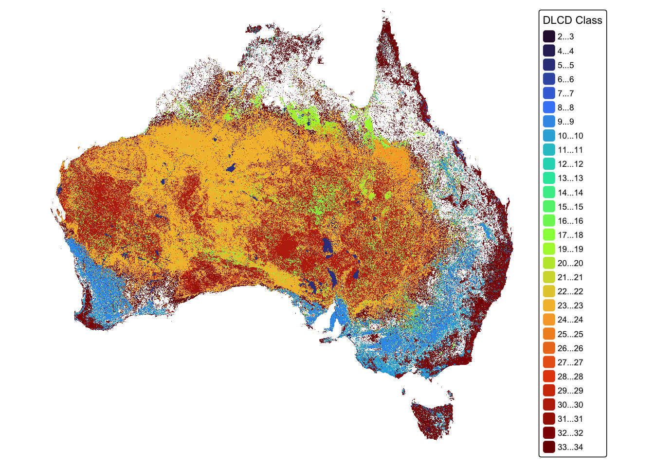
The DLCD layer thematically illustrates Australian land cover that is divided into 34 different land cover classes. tmap is limited to displaying 30 classes (see warning message above) and so the map combines some of the classes together. This is not a problem for analysing the data and only affects the way some of the classes are displayed.
Each of the 34 classes is identified by a number. Rainfed crops are identified by the number 8.
A full description of each class and the methodology used to derive the DLCD map is provided in the DLCD Report published by Geoscience Australia, and available through the DLCD dataset download page.
Next, we plot the mean EVI trends raster:
tm_shape(mean_evi) +
  tm_raster("EVI",
      col.scale = tm_scale_continuous(
          values = "pu_gn_div",
          limits = c(-0.02, 0.02),        # Limit the scale to improve visibility
          outliers.trunc = c(TRUE, TRUE)  # Remove outliers (values beyond limits set above)
                   ),
      col.legend = tm_legend(
          title = "EVI trends",
          position = tm_pos_out(cell.h = "right", cell.v = "center"),
          orientation = "portrait"
                   )
  ) +
  tm_layout(frame = FALSE)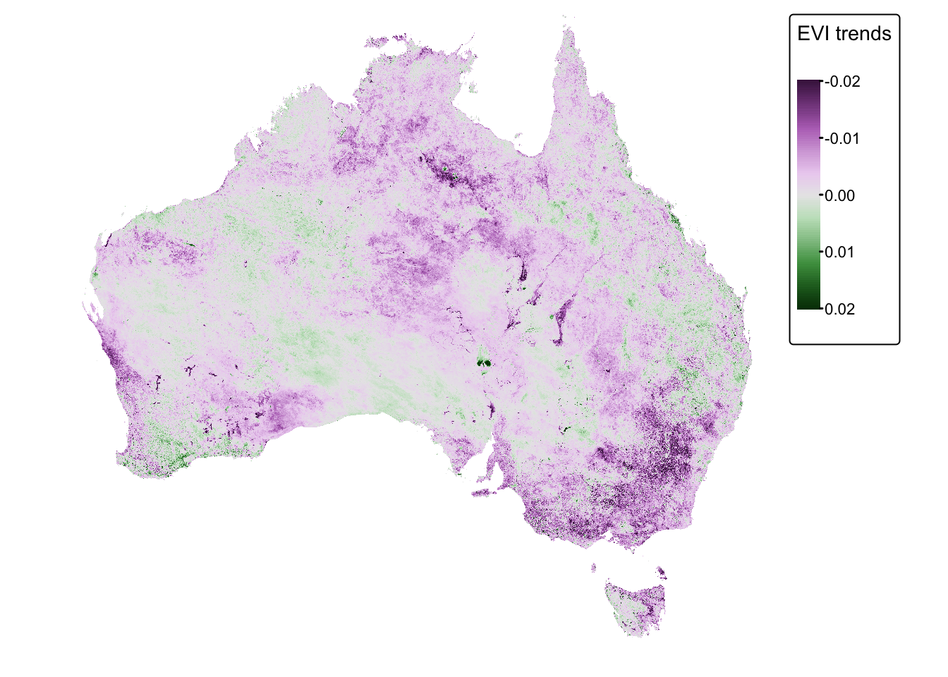
In the above map, positive values (green) represent grid cells where vegetation cover has increased over the observation period (i.e., 2000 to 2008). Conversely, negative values (purple) represent grid cells where vegetation cover has decreased. A value of zero (gray) indicates no change.
Isolate rainfed crops
In this step we will use the ifel() conditional (i.e.,
if-else) function to produce a new raster layer that stores
mean EVI values for rainfed crops. EVI values for all other DLCD classes
are reclassified to NA.
# Check that both rasters have the same extent and resolution.
if (!compareGeom(dlcd_classes, mean_evi, stopOnError = FALSE)) {
  stop("The rasters do not have the same geometry. Please align them first.")
}

# For cells where the DLCF raster equals 8,
# assign the corresponding value from the EVI raster;
# Otherwise, set the cell to NA.
rainfed_crops <- ifel(dlcd_classes == 8, mean_evi, NA)

#Change the name of the layer to "EVI"
names(rainfed_crops) <- "EVI"

# Print a summary of the result
print(rainfed_crops)
## class : SpatRaster
## dimensions : 14902, 19161, 1 (nrow, ncol, nlyr)
## resolution : 0.002349, 0.002349 (x, y)
## extent : 110, 155.0092, -45.0048, -10 (xmin, xmax, ymin, ymax)
## coord. ref. : lon/lat WGS 84 (EPSG:4326)
## source(s) : memory
## varname : DLCDv1_Class
## name : EVI
## min value : -0.08947342
## max value : 0.07360858Plot the rainfed_crops layer:
rainfed_map <-
  tm_shape(rainfed_crops) +
    tm_raster("EVI",
        col.scale = tm_scale_continuous(
          values = "pu_gn_div",
          limits = c(-0.02, 0.02),        # limit the scale to improve visibility
          outliers.trunc = c(TRUE, TRUE)  # remove outliers (values beyond limits set above)
                    ),
         col.legend = tm_legend(
           title = "EVI trends in \nrainfed crops",
           position = tm_pos_out(cell.h = "right", cell.v = "center"),
           orientation = "portrait"
                    )
  ) +
  tm_layout(frame = FALSE)

# Plot coastline for visual clarity
rainfed_map + tm_shape(aus_coast_proj) + tm_borders("lightgray") 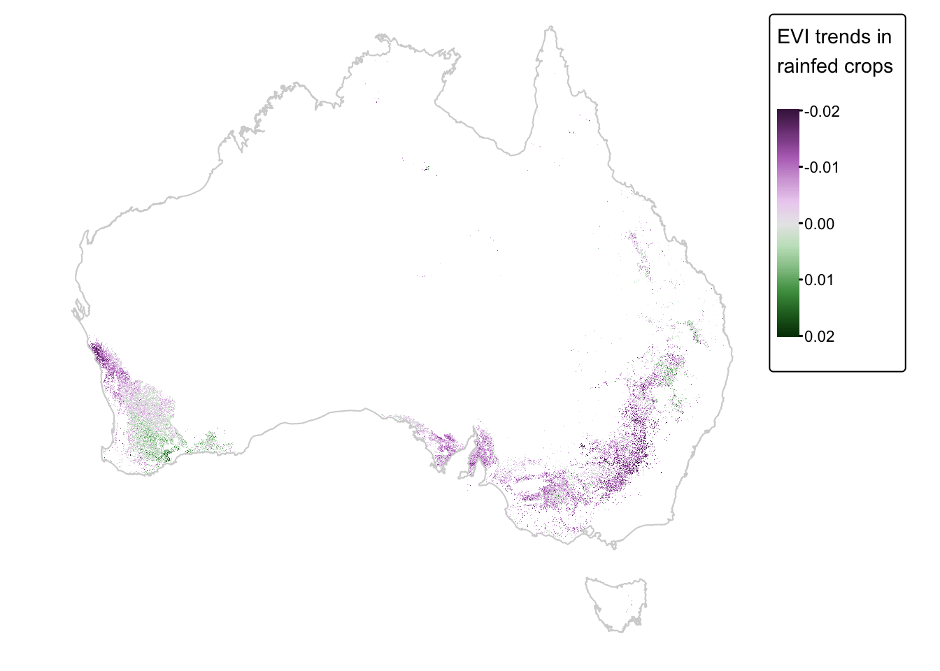
Crop to NSW boundary
To crop the rainfed_crops raster to the extent of the
state of NSW, we will use the crop() and
mask()functions in terra. A vector dataset
representing the NSW state boundary is provided.
The next chunk of code loads the NSW boundary data:
# Read in shapefile
nsw_bnd <- read_sf("./data/data_crops/vector/shapefile/bnd_nsw_AGD66.shp")

# Plot shapefile for quick visual inspection
tm_shape(nsw_bnd) +
      tm_fill() + tm_borders() +
      tm_layout(frame = FALSE)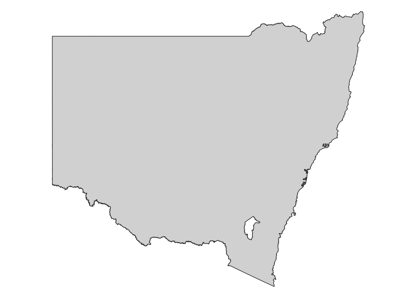
## Simple feature collection with 1 feature and 13 fields
## Geometry type: POLYGON
## Dimension:     XY
## Bounding box:  xmin: 140.998 ymin: -37.50643 xmax: 153.6375 ymax: -28.15893
## Geodetic CRS:  AGD66
## # A tibble: 1 × 14
##   OBJECTID FEATTYPE STATE FEATREL    ATTRREL    PLANACC SOURCE        CREATED
##      <dbl> <chr>    <chr> <date>     <date>       <int> <chr>         <date>
## 1        9 Mainland NSW   2004-11-16 2004-11-16    9999 GEOSCIENCE A… 2006-05-09
## # ℹ 6 more variables: RETIRED <date>, PID <dbl>, SYMBOL <int>,
## #   SHAPE_Leng <dbl>, SHAPE_Area <dbl>, geometry <POLYGON [°]>
Based on the above summary, the data is projected in geographic
coordinates that are referenced to the AGD66 datum. Before we proceed
with cropping, we need to reproject the data so that its CRS matches
that of the rainfed_crops raster:
# Transform to EPSG:4326
nsw_bnd_proj <- st_transform(nsw_bnd, st_crs(rainfed_crops))

# Plot shapefile for quick visual inspection
tm_shape(nsw_bnd_proj) +
      tm_fill() + tm_borders() +
      tm_layout(frame = FALSE)
Given that the CRS transformation only changes the datum, no actual warping of the vector features occurs and so the two NSW maps above look identical. To confirm that the CRS transformation has occurred:
## Simple feature collection with 1 feature and 13 fields
## Geometry type: POLYGON
## Dimension:     XY
## Bounding box:  xmin: 140.9993 ymin: -37.50487 xmax: 153.6386 ymax: -28.15734
## Geodetic CRS:  WGS 84
## # A tibble: 1 × 14
##   OBJECTID FEATTYPE STATE FEATREL    ATTRREL    PLANACC SOURCE        CREATED
## *    <dbl> <chr>    <chr> <date>     <date>       <int> <chr>         <date>
## 1        9 Mainland NSW   2004-11-16 2004-11-16    9999 GEOSCIENCE A… 2006-05-09
## # ℹ 6 more variables: RETIRED <date>, PID <dbl>, SYMBOL <int>,
## #   SHAPE_Leng <dbl>, SHAPE_Area <dbl>, geometry <POLYGON [°]>
Indeed, Geodetic CRS is now listed as WGS 84.
Crop the rainfed_crops raster:
# Convert sf POLYGON geometry object to terra SpatVector object
nsw_bnd_vect <- vect(nsw_bnd_proj)

# Crop rainfed_crops raster
rainfed_nsw = crop(rainfed_crops, nsw_bnd_vect)
rainfed_nsw_final = mask(rainfed_nsw, nsw_bnd_vect)
Plot the cropped raster:
rainfed_map <-
  tm_shape(rainfed_nsw_final) +
    tm_raster("EVI",
        col.scale = tm_scale_continuous(
          values = "pu_gn_div",
          limits = c(-0.02, 0.02),        # limit the scale to improve visibility
          outliers.trunc = c(TRUE, TRUE)  # remove outliers (values beyond limits set above)
                    ),
         col.legend = tm_legend(
           title = "EVI trends, \nRainfed Crops",
           position = tm_pos_out(cell.h = "right", cell.v = "center"),
           orientation = "portrait"
                    )
  ) +
  tm_layout(frame = FALSE)

# Plot coastline for visual clarity
rainfed_map + tm_shape(nsw_bnd_proj) + tm_borders("lightgray") 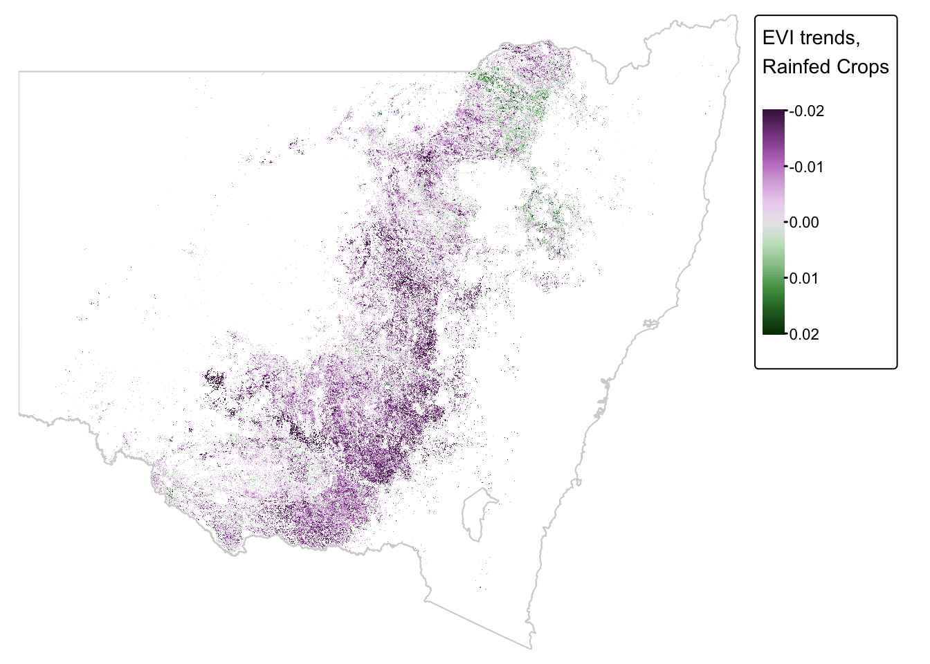
Map change in crops
In this step we will create an interactive map that shows the EVI trends for rainfed crops in NSW. The map will also include the NSW boundary polygon and the location of major cities and towns along with their names.
A list of cities and towns along with their lat/long coordinates, is provided in a CSV file:
# Read CSV file with cities and towns
nsw_cities <-
  read.csv("./data/data_crops/vector/txt/NSW_Cities.csv",
           header = TRUE, sep = ","
          )

# Print the first rows
head(nsw_cities)
To convert the tabular data frame into a spatial sf object:
# Convert the data frame to an sf object.
# Here, 'coords' specifies the names of the coordinate columns.
# 'crs' is defined as 4326 (WGS84),
nsw_cities_points <-
  st_as_sf(nsw_cities, coords = c("POINT_X", "POINT_Y"), crs = 4326)

# Print the sf object to check the result
print(nsw_cities_points)
## Simple feature collection with 14 features and 2 fields
## Geometry type: POINT
## Dimension: XY
## Bounding box: xmin: 146.9239 ymin: -36.07494 xmax: 153.542 ymax: -28.17561
## Geodetic CRS: WGS 84
## First 10 features:
## FID NAME geometry
## 1 0 ALBURY POINT (146.9239 -36.07494)
## 2 1 CENTRAL COAST POINT (151.3714 -33.42979)
## 3 2 ORANGE POINT (149.1 -33.28309)
## 4 3 BATHURST POINT (149.5813 -33.41736)
## 5 4 NOWRA POINT (150.6003 -34.88422)
## 6 5 NEWCASTLE POINT (151.7845 -32.92779)
## 7 6 TAMWORTH POINT (150.929 -31.09048)
## 8 7 TWEED HEADS POINT (153.542 -28.17561)
## 9 8 COFFS HARBOUR POINT (153.1135 -30.29626)
## 10 9 PORT MACQUARIE POINT (152.9089 -31.43084)We are now ready to make our final map:
# Set tmap to dynamic maps
tmap_mode("view")

# Draw map
map_crops <-
  tm_shape(rainfed_nsw_final) +
    tm_raster("EVI",
      col.scale = tm_scale_intervals(           # Custom breaks
        values = c("red", "grey", "green"),     # Define colours
        breaks = c(-0.02, -1e-6, 1e-6, 0.02),   # Tiny gap around 0 isolates zero values.
        labels = c("loss", "no change", "gain") # Legend labels
                ),
       col.legend = tm_legend(
         title = "EVI trends in \nrainfed crops",
         position = tm_pos_out(cell.h = "right", cell.v = "center"),
         orientation = "portrait"
                )
  )

map_crops2 <-
  map_crops+ tm_shape(nsw_bnd_proj) + tm_borders("lightgray")

map_crops2 + tm_shape(nsw_cities_points) +
    tm_symbols(shape = 22, size = 0.6, fill = "white") +                  # Show as squares
    tm_labels("NAME", size = 0.8, col = "black", xmod = unit(0.1, "mm"))  # Add labels
The above map is interactive and so feel free to zoom in/out and inspect different parts of NSW. Values in red represent grid cells where vegetation cover (in this case rainfed crops) has decreased over the observation period between 2000 and 2008.
Values in green represent grid cells where vegetation cover has increased. The map indicates that in most parts of NSW land cover by rainfed crops has decreased and this is in line with changes in precipitation patterns over the last few decades (i.e., less rainfall).
Summary
In this practical we used publicly available gridded weather data from the Bureau of Meteorology (BOM) and land cover data from Geoscience Australia (GA) to explore how precipitation and temperature patterns have changed over the past 30 years in Australia, and how these changes might have affected rainfed crops in NSW.
The analyses showcased a range of functions from the sf and terra packages. In addition, this practical also introduced a number of tmap functions that control the way map colour scales are constructed.
List of R functions
A brief summary of R functions used in this practical is provided below:
base R functions
c(): concatenates its arguments to create a vector, which is one of the most fundamental data structures in R. It is used to combine numbers, strings, and other objects into a single vector.head(): returns the first few elements or rows of an object, such as a vector, matrix, or data frame. It is a convenient tool for quickly inspecting the structure and content of data.print(): outputs the value of an R object to the console. It is useful for debugging and ensuring that objects are displayed correctly within functions.read.csv(): imports data from a CSV file into R by converting it into a data frame. It is widely used for reading external datasets into R with customizable options for headers, delimiters, and missing values.seq(): generates regular sequences of numbers based on specified start, end, and increment values. It is essential for creating vectors that represent ranges or intervals.
grid functions
unit(): constructs unit objects that specify measurements for graphical parameters, such as centimeters or inches. It is often used in layout and annotation functions for precise control over plot elements.
sf functions
read_sf(): reads vector spatial data from formats like shapefiles or GeoJSON into R as an sf object. It simplifies the import of geographic data for spatial analysis.st_as_sf(): converts various spatial data types, such as data frames or legacy spatial objects, into an sf object. It enables standardised spatial operations on the data.st_bbox(): computes the bounding box of an sf object, representing the minimum rectangle that encloses the geometry. It is useful for setting map extents and spatial limits.st_crs(): retrieves or sets the coordinate reference system (CRS) of an sf object. It is essential for ensuring that spatial data align correctly on maps.st_transform(): reprojects spatial data into a different coordinate reference system. It ensures consistent spatial alignment across multiple datasets.st_union(): merges multiple spatial features into a single combined geometry. It is useful for dissolving boundaries and creating aggregate spatial features.
terra functions
compareGeom(): compares the geometry, extent, resolution, and coordinate system of two spatial objects. It is used to ensure that spatial datasets are compatible for further processing.crs(): retrieves or sets the coordinate reference system for spatial objects such as SpatRaster or SpatVector. It is essential for proper projection and alignment of spatial data.crop(): trims a raster to a specified spatial extent. It is used to focus analysis on a region of interest within a larger dataset.global(): computes summary statistics, such as mean or sum, for the cells in a SpatRaster across its entire extent. It provides a quick overview of the raster data’s overall characteristics.ifel(): performs element-wise conditional operations on raster data, similar to an if-else statement. It creates new rasters based on specified conditions.mask(): applies a mask to a raster using a vector or another raster, setting cells outside the desired area to NA. It is useful for isolating specific regions within a dataset.names(): gets or sets the names of layers within a SpatRaster object. It facilitates easier reference and manipulation of individual raster layers.project(): reprojects spatial data from one CRS to another, enabling alignment of datasets. It is essential for working with spatial data from different sources.rast(): creates a new SpatRaster object or converts data into a raster format. It is the entry point for handling multi-layered spatial data in terra.vect(): converts various data types into a SpatVector object for vector spatial analysis. It supports points, lines, and polygons for versatile spatial data manipulation.values(): retrieves or assigns the cell values of a SpatRaster. It allows direct manipulation of the underlying data in the raster.
tmap functions
tm_borders(): draws border lines around spatial objects on a map. It is often used in combination with fill functions to delineate regions clearly.tm_compass(): adds a compass element to a map to indicate orientation. It offers customizable styles and positions for clear directional reference.tm_crs(): sets or retrieves the coordinate reference system for a tmap object. It ensures that all spatial layers are correctly projected.tm_facets_wrap(): creates a faceted layout by splitting a map into multiple panels based on a grouping variable. It is useful for comparing maps across different time periods or categories.tm_fill(): fills spatial objects with color based on data values or specified aesthetics in a tmap. It is a key function for thematic mapping.tm_graticules(): adds graticule lines (latitude and longitude grids) to a map, providing spatial reference. It improves map readability and context.tm_labels(): adds text labels to map features based on specified attributes in tmap. It is useful for annotating spatial data to improve map readability.tm_layout(): customises the overall layout of a tmap, including margins, frames, and backgrounds. It provides fine control over the visual presentation of the map.tm_legend(): customises the appearance and title of map legends in tmap. It is used to enhance the clarity and presentation of map information.tm_pos_out(): positions map elements, such as legends or scale bars, outside the main map panel. It helps declutter the map area for a cleaner display.tm_raster(): adds a raster layer to a map with options for transparency and color palettes. It is tailored for visualizing continuous spatial data.tm_scale_continuous(): applies a continuous color scale to a raster layer in tmap. It is suitable for representing numeric data with smooth gradients.tm_scale_continuous_sqrt(): applies a square root transformation to a continuous color scale in tmap. It is useful for visualizing data with skewed distributions.tm_scale_categorical(): applies a categorical color scale to represent discrete data in tmap. It is ideal for mapping data that fall into distinct classes.tm_scale_intervals(): creates a custom interval-based color scale for a raster layer in tmap. It enhances visualization by breaking data into meaningful ranges.tm_scalebar(): adds a scale bar to the map to indicate distance. It can be customised in terms of breaks, text size, and position.tm_shape(): defines the spatial object that subsequent tmap layers will reference. It establishes the base layer for building thematic maps.tm_symbols(): adds point symbols to a map with customisable shapes, sizes, and colors based on data attributes. It is useful for plotting locations with varying characteristics.tm_title(): adds a title and optional subtitle to a tmap, providing descriptive context. It helps clarify the purpose and content of the map.tmap_arrange(): arranges multiple tmap objects into a single composite layout. It is useful for side-by-side comparisons or dashboard displays.tmap_mode(): switches between static (“plot”) and interactive (“view”) mapping modes in tmap. It allows users to choose the most appropriate display format for their needs.